Accurate loop calling for 3D genomic data with cLoops

Abstract

Motivation

Sequencing-based 3D genome mapping technologies can identify loops formed by interactions between regulatory elements hundreds of kilobases apart. Existing loop-calling tools are mostly restricted to a single data type, with accuracy dependent on a predefined resolution contact matrix or called peaks, and can have prohibitive hardware costs.

Results

Here, we introduce cLoops (‘see loops’) to address these limitations. cLoops is based on the clustering algorithm cDBSCAN that directly analyzes the paired-end tags (PETs) to find candidate loops and uses a permuted local background to estimate statistical significance. These two data-type-independent processes enable loops to be reliably identified for both sharp and broad peak data, including but not limited to ChIA-PET, Hi-C, HiChIP and Trac-looping data. Loops identified by cLoops showed much less distance-dependent bias and higher enrichment relative to local regions than existing tools. Altogether, cLoops improves accuracy of detecting of 3D-genomic loops from sequencing data, is versatile, flexible, efficient, and has modest hardware requirements.

Availability and implementation

cLoops with documentation and example data are freely available at: https://github.com/YaqiangCao/cLoops.

Supplementary information

Supplementary data are available at Bioinformatics online.

1 Introduction

Three-dimensional genomic interactions are essential for genome organization which provides vital biological function. A loop is classified as two genomic loci that are linearly distant but have a significantly higher contact frequency than random noise (Yu and Ren, 2017). CTCF (Handoko et al., 2011; Splinter et al., 2006) and cohesin (Kagey et al., 2010; Rao et al., 2017) are thought to anchor most of loops on chromatins which could help enhancers find their target promoters (Dowen et al., 2014), and YY1 is considered responsible for many enhancer-promoter loops (Weintraub et al., 2017). Identification of loops, especially enhancer-promoter loops, may reveal direct transcriptional regulatory roles of distal regulatory elements.

Loops can be identified at near-kilobase resolution (Yu and Ren, 2017). With the development of high-resolution chromosome conformation capture (3C) derived high-throughput sequencing methods, it is possible to identify loops genome-wide (Dekker, 2016). ChIA-PET (Fullwood et al., 2009; Tang et al., 2015) identifies high-resolution interactions between regulatory elements using target antibodies. Hi-C (Lieberman-Aiden et al., 2009; Rao et al., 2014) maps all possible genomic interactions in an unbiased manner. With deep sequencing [i.e. 6.5 billion total paired-end tags (PETs)], in situ Hi-C can achieve 1 kb level resolution (Rao et al., 2014), which enables high-resolution detection of loops. Meanwhile, HiChIP (Mumbach et al., 2016) which combines the advantages of ChIP and in situ Hi-C, uses fewer input cells than ChIA-PET and attains higher signal-to-background enrichment than in situ Hi-C, could provide high-resolution data for loop calling. A new method to identify short- and long-range interactions called Trac-looping (Lai et al., 2018) was developed recently that uses transposon linkers prior to fragmentation and ligation, capturing the interactions between open chromatin regions. Each different technology generates huge datasets and has major computational demands, creating a need for efficient and versatile analysis tools.

Finding long-range loops from 3D genomic interaction data is a computational task equivalent to finding peaks from ChIP-seq data, becoming a basic analysis step prior to biological interpretation. Due to data-type specific technology derived biases and different resolutions, many loop-calling tools have been designed. With Hi-C, no algorithm is yet considered to be a golden standard (Forcato et al., 2017). Recently developed loop-calling tools for ChIA-PET data such as Mango (Phanstiel et al., 2015) and MICC (He et al., 2015)—implemented in ChIA-PET2 (Li et al., 2016)—often start with peak calling, then use exhaustive combinations of peaks to find candidate loops, including modeling the relation between PETs and distances, and the peaks’ size and depth, which altogether increases data processing time. Importantly, uncertainty in analysis arises when modeling the PETs and distance relations, as different fitting functions and parameters can lead to different loop identification. There is also a problem of bias if the interacting loci forming loops may exist outside of peak regions, which would bias the background used in significance estimations. Correspondingly, we have noticed these tools fail to call loops accurately for data containing broad peaks, such as H3K4me1 ChIA-PET data. The hardware requirements for loop calling from Hi-C data present another major limitation. For example, the major Hi-C loop-calling tool HiCCUPS from Juicer (Durand et al., 2016) requires NVIDIA graphics processing units (GPUs) which are not widely equipped on average servers, and the central processing unit (CPU)-version of Juicer may ignore distant interactions (Supplementary Fig. S1A). Due to huge PET numbers, loop-calling tools for Hi-C usually have high RAM usage, according to estimates in a Hi-C tools comparative study, contact matrix-based tools like Fit-Hi-C (Ay et al., 2014) and GOTHiC (Mifsud et al., 2017) require more than 512 GB of RAM for a 5 kb resolution contact matrix (Forcato et al., 2017), making loop calling on a 1 kb high-resolution contact matrix from deep sequencing impossible. Currently, to our knowledge, there is only one targeted loop-calling tool for HiChIP data, hichipper (Lareau and Aryee, 2018). The basic loop-calling procedure of hichipper is very similar to Mango and ChIA-PET2; it first uses MACS (Zhang et al., 2008) to call peaks from the HiChIP data with custom background models and then identify loops depends on Mango. The method for calling loops from Trac-looping data is the same as in hichipper, thus the biases can also be inherited from those in Mango.

To avoid biases, present in the existing loop-calling tools and to provide a low-computational-cost and universal solution for 3D-genome mapping data we developed a new tool: cLoops (‘see loops’). cLoops is a versatile loop-calling tool for multiple types of 3D-genome mapping data. It uses an unbiased clustering algorithm to find candidate loops, coupled with a permutated local background method for estimation of a candidate loop’s statistical significance. We show the advantages of cLoops over existing state-of-the-art loop-calling tools by comparisons with ChIA-PET, Hi-C, HiChIP and Trac-looping data. Briefly, (i) cLoops is easy to use, having only two essential input parameters, for which we provided predetermined default values for ChIA-PET, Hi-C, HiChIP and Trac-looping data. (ii) cLoops can run efficiently on personal computers (PCs) and accurately identify loops for both sharp-peak and broad-peak data. (iii) Compared to other tools, performance was distinguished by cLoops’ uniquely identified loops that showed more easily distinguishable signals within their neighboring regions, cLoops identified more distant loops from Hi-C and HiChIP data and showed higher overlap with ChIA-PET loops without any specific setting for calling distant loops. (iv) cLoops’ reliability was not affected by sequencing depth, with equivalent performance in both deep and unsaturated HiChIP sequencing data. (v) cLoops is not tied to any particular experimental method, therefore, is applicable to 3D-genome mapping data generated by future experimental methods, as long as there are data with enriched interactions detectable on an interaction heatmap.

2 Materials and methods

2.1 Public data used

Public datasets used were summarized in Supplementary Table S1.

2.2 Data pre-processing

Raw FASTQ files of ChIA-PET data were pre-processed to mapped de-duplicated intra-chromosomal PETs by Mango (Phanstiel et al., 2015). ChIA-PET2 pipeline was used to call loops with ChIA-PET2 (Li et al., 2016). Raw FASTQ files of merged cohesin HiChIP data were pre-processed to PETs by HiCUP (v0.5.4) (Wingett et al., 2015). Raw FASTQ files of HiC data and two cohesin HiChIP replicates data were pre-processed by HiC-Pro (v2.10.0) (Servant et al., 2015). BEDPE files of resting CD4⁺ Trac-looping data mapped to hg19 were obtained from Gene Expression Omnibus and replicates were merged. All raw data except Trac-looping were mapped to genome version hg38. To avoid bugs in some tools like Mango, only intra-chromosomal PETs in chr1-22 and chrX were used to call loops. Pre-processing specifically required by some tools were addressed in Supplementary Methods.

2.3 Aggregate peak analysis for loops comparison

To show the enrichment of global mean profiles of all called loops with their nearby regions for the Hi-C and HiChIP data, Juicer aggregate peak analysis (APA) (Durand et al., 2016) (with parameters –n 0 –w 5 –r 5000 –u or –n 0 –w 5 –r 10000 –u) was used to get the view of centerNormedAPA and Peak to Mean (P2M) score (indicating the enrichment of loops compared to nearby regions) was used. Here, –n 0 was used to analyze all loops without filtering out loops that are close to the diagonal line of the input contact matrix. For ChIA-PET data, -n was set to 0, 10, 20 and 30 (default), respectively, for comparison. When performing APA for Trac-looping loops, 1 kb resolution was used for both Trac-looping and Hi-C data. The centerNormedAPA heatmaps output by Juicer APA were used for genome-wide visualized comparison. In a centerNormedAPA heatmap, loops are positioned at the heatmap center, which indicates the loops enrichment comparing to nearby regions. Higher interacting regions not in the center of heatmap may indicate poor global quality for loops called. We obtained centerNormedAPA matrix from gw/enhancement.txt of Juicer APA’s output. We mainly used P2M score as global quality indicator of loops due to following reasons: (i) According to Juicer (Durand et al., 2016) documentation, the definition of P2M score is the ratio of the central pixel to the mean of the remaining pixels, which indicates the enrichment of interactions in loop regions against nearby background. We also compared Peak to Lower Left (P2LL) score (P2LL score was suggested by Juicer APA guide) and its related ZscoreLL, which is the ratio of the central pixel to the mean of pixels in the lower-left corner. (ii) If there are too many loops fed to Juicer APA, for example, 748, 786 GM12878 Hi-C loops output by GOTHiC, Juicer APA will crash without generating gw/measures.txt file which record global P2LL score and other indicators. Meanwhile, there is always a file named ‘enhancement.txt’ recording P2M score for every loop when feeding loops to Juicer APA one chromosome at a time.

2.4 Cumulative aggregate peak analysis

The cumulative aggregate peak analysis (CAPA) was carried out according to Mango (Phanstiel et al., 2015) to evaluate loops quality called from ChIA-PET data using Hi-C. Briefly, to generate CAPA plots, we ranked loops by P-values or false discovery rate (FDR) and calculated a recommend P2LL aggregate peaks analysis score by the command of APA in Juicer (Durand et al., 2016) in a cumulative process adding 100 ChIA-PET loops at a time when more than 1000 loops are present, or else 20 at a time.

2.5 Visualization of example loops

Juicebox (Durand et al., 2016) was used to show loops in 5 kb resolution. WashU Epigenome Browser (Li et al., 2019) was used to closely inspect PETs distribution around loops without resolution limit.

2.6 Input and output of cLoops

cLoops takes BEDPE format mapped PET data generated by preprocessing software like HiC-Pro (Servant et al., 2015) as input and generates a tab-delimited loop file that contains all potential loops (with more PETs than required $\mathit{minPts}$⁠) and its significance, with significant loops marked 1. Converted loop file for visualization in WashU Epigenome Browser (Li et al., 2019) or Juicebox (Durand et al., 2016) could also be generated if certain parameters are given.

3 Results

3.1 cDBSCAN algorithm

DBSCAN (Density-Based Spatial Clustering of Applications with Noise) (Ester et al., 1996) is one of the most widely used unsupervised clustering algorithms. DBSCAN contains two key parameters: $\mathit{eps}$ defines the distance within which two points are classified as neighbors and $\mathit{minPts}$ defines the smallest number of points required in a cluster. It has been introduced for ChIA-PET by taking all PETs as 2D points, and identifying significant clusters in 2D space as potential loops (Chepelev et al., 2012). The density-based principle, tolerance of noise and unsupervised auto-determination of the number of clusters, theoretically make DBSCAN very suitable for finding candidate loops from 3D genomic interaction data. However, the original DBSCAN algorithm runs very slowly for ChIA-PET and Hi-C data [with complexity of O(N²) without any optimization for neighbor search, N is the number of points]. For example, if implemented with the C programming language-based KD-Tree for neighbor search [named kDBSCAN, with complexity of O(Nlog(N)), Supplementary Methods] on a computer with a 3.2 GHz CPU (see the detailed configuration of computers used in Supplementary Information), the average time of five runs for kDBSCAN is about 32 s (⁠$\mathit{eps}=750,\mathit{minPts}=5$⁠) to finish clustering on 99 674 PETs in the smallest human autosome (chromosome 21) from GM12878 CTCF ChIA-PET data (Supplementary Table S1) and about 1.1 h (⁠$\mathit{eps}=5000,\mathit{minPts}=20$⁠) for 2 268 476 PETs in chromosome 21 from GM12878 Hi-C data (Supplementary Table S1). Although DBSCAN has been implemented in TADLib for interaction block analysis within topological associated domains (TADs) (Wang et al., 2015), so far no tools have implemented it for loop calling, or to determine the loop-calling effectiveness or significance. We thus first propose a specific improvement to DBSCAN (named cDBSCAN for cLoops’ DBSCAN) for 2D data, by introducing an indexing method for noise reduction and neighbor search (see toy example data in Fig. 1A for illustration of the algorithm).

Fig. 1.

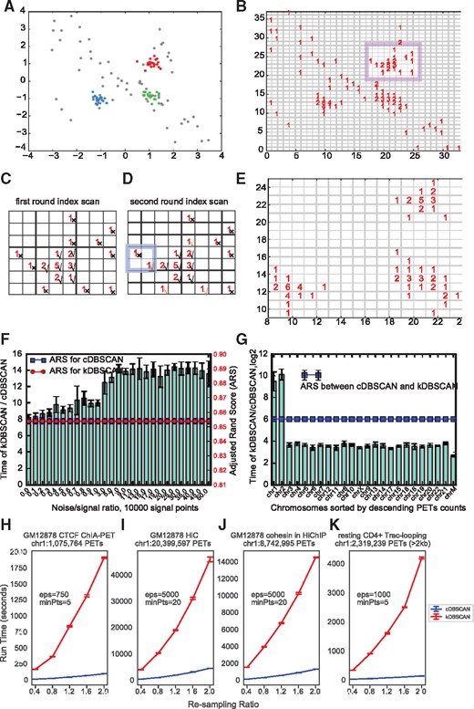
The cDBSCAN algorithm. (A) A toy example of the simulated test data, mainly three clusters, centered at (−1, −1), (1, −1) and (1, 1) with $\mathit{std}=0.2$⁠, a total of 60 signal points and 60 noise points. Noise is generated randomly and marked as gray points. (B) Indexing result, each point is attached to a square with side length of $\mathit{eps}$⁠, which equals to$\mathit{std}$ here, the numbers in the squares indicate the number of points indexed in that square. The highlighted region is used to represent detected noise. (C) An example of first round of noise removal, the region is highlighted in B. For an $\mathit{eps}$ square, scan the nearby eight squares, if the total number of nearby points is less than required $\mathit{minPts}$ which is five here, then the index square is marked as noise. A noise index is marked by a cross, while a signal index is marked by a checkmark. (D) Second round of noise removal for the same region in C, for a noise index detected in C, if one of its neighbor square indexes is a signal index, then it is re-marked to a signal index. Examples are marked by orange checkmarks. The highlighted region is an example and an outer index that is not re-marked as signal index. (E) An example of indexed $\mathit{eps}$ square after noise removal. (F) Comparison of running CPU time at different noise/signal ratio based on 10 repeats for the simulation data. Left y-axis marks the bars for running time ratios; right y-axis marks the lines for ARS. The two ARS are exactly the same. (G) Comparison of running CPU time using real GM12878 CTCF ChIA-PET data (GSM1872886) for each chromosome based on five repeats, with $\mathit{eps}=750$ and $\mathit{minPts}=5$⁠. Error bars denote standard deviations. (H–K) Re-sampling to bootstrap run time of cDBSCAN and kDBSCAN for GM12878 CTCF ChIA-PET chr1 (H), GM12878 Hi-C chr1 (I), GM12878 cohesin HiChIP chr1 (J) and resting CD4⁺ cell Trac-looping chr1 data (K). The parameters to run cDBSCAN and PETs numbers were annotated in the figures, except for Trac-looping, all cis-PETs in chr1 were used and for Trac-looping only the PETs with distance > 2 kb were used. All plots were based on four runs for each re-sampling ratio

cDBSCAN also has two key parameters with the same meaning as those in DBSCAN: $\mathit{eps}$ and $\mathit{minPts}$⁠. For 3C-based genome-wide sequencing data like ChIA-PET, HiChIP and Hi-C data, the Manhattan distance (also known as city block distance) is suitable for measuring the absolute position difference for two PETs. Unless specifically mentioned, the distance measurements hereafter refer to Manhattan distance. For the 2D dataset $D\left(X,Y\right)$in the cDBSCAN algorithm, X and Y can be integer or float values, but for loop calling, they are all both integers corresponding to genomic coordinates. We mark the minimum $X,Y$ as $\mathit{minX},\mathit{min}Y$ for the 2D space. cDBSCAN indexes each point $\left(X_i, Y_i\right)$ as

$${\mathit{Index}}_i=\left(\mathit{int}\left(\frac{X_i-\mathit{minX}}{\mathit{eps}}\right),\mathit{int}\left(\frac{Y_i-\mathit{minY}}{\mathit{eps}}\right)\right)$$

which means each point is assigned to a square whose side length is $\mathit{eps}$ (0.2 is used for the toy example) (Fig. 1B) and j marks the index id of the point id i. For an indexed $\mathit{eps}$ square, if the square together with its surrounding eight squares contains points fewer than $\mathit{minPts}$ (five is used for the toy example), then it is defined as a noise index. We highlight a region in Figure 1B (also used in Fig. 1C and D) to show how cDBSCAN removes noise. There are two rounds of index scanning in cDBSCAN to detect noise. The first round finds all potential noise indexes (marked by a cross in Fig. 1C), and the second round only searches previously detected noise indexes (cross marked indexes). If there is a first-round signal index (marked by checkmarks) in any of its eight neighbors, then it is marked as a signal index (Fig. 1D orange checkmarks). The highlighted region in Figure 1D is an example showing an outer index that is not re-marked is a signal index and a closer index that is re-marked as a signal index. The idea benefits from k-Nearest Neighbor algorithm—that is, if all neighbors are noise then the index is noise. A signal index detected in the second-round search is not counted as a signal index when a noise is corrected back to a signal (Fig. 1D). This indexing process reduces search space (Fig. 1E). After indexing, the clustering is performed the same as DBSCAN for the remaining points but uses the $3e\mathit{ps}\times 3e\mathit{ps}$ squares for neighbor search.

We first evaluated the performance of cDBSCAN by comparing to a C coded KD-tree for neighbor search (termed it kDBSCAN as mentioned above) (Supplementary Methods) using simulated data. We set 10 000 signal points of 100 clusters and different noise/signal ratios for the simulation data (Supplementary Methods). cDBSCAN coded in pure Python gives the exact same result as kDBSCAN (measured by Adjusted Rand Score (ARS)) (Hubert and Arabie, 1985). ARS measures the similarity between clustering results ranging from −1.0 to 1.0, with 0 indicating random labeling and 1 a perfect match. cDBSCAN had improved speed (8–16-fold) with about twice RAM usage (Supplementary Fig. S1B), without considering the inefficiency of Python compared to C in simulation data (Fig. 1F). We also validated the speed increase on real GM12878 CTCF ChIA-PET data and found a ∼8–1000-fold increases (Fig. 1G) with acceptable RAM usage increase (Supplementary Fig. S1C). Comparing to kDBSCAN $O\left(\mathit{Nlog}\left(N\right)\right)$ complexity, cDBSCAN is approximate $O\left(N\right)$ complexity in most ideal situation, which is further validated by running cDBSCAN for the PETs in chromosome 1 for CTCF ChIA-PET (Fig. 1H), GM12878 Hi-C (Fig. 1I), GM12878 cohesin HiChIP (Fig. 1J) and the Trac-looping data (Fig. 1K) as the run time increases nearly linearly when the number of PETs increases.

3.2 Overview of cLoops

Based on cDBSCAN we built cLoops (see loops) as a two-step loop-calling algorithm. cLoops is a light-weight tool coded in pure Python with dependence on only a few commonly used and well-maintained packages such as scipy, numpy, pandas, joblib and seaborn, some additional scripts in cLoops for data format conversion that required by some users, require other tools such as juicer tools, bedtools, bgzip and tabix. The first step takes mapped PET data in BEDPE format rather than contact matrix and uses cDBSCAN to find candidate loops, without binning PETs into a specific assigned resolution contact matrix (as usually occurs with Hi-C loop-calling tools such as Fit-Hi-C) or identifying peaks from PETs which are then used to find significant combinations (as needed by common ChIA-PET loop-calling tools such as Mango), enabling precise detection of loop boundaries from mapped PETs. In the second step, candidate loops’ significance are estimated by comparing their number of PETs to respective permuted local backgrounds (PLBs). The overview of data processing steps of cLoops is demonstrated in Supplementary Figure S1D. We show the algorithmic details of cLoops using GM12878 CTCF ChIA-PET data as follows.

First, each intra-chromosomal PET is mapped to a 2D space by taking the middle coordinate of the left-end tag as the X-coordinate, and the middle coordinate of the right-end tag as Y-coordinate into $\left(X_i,Y_i\right)$ where i indicates the PET id (Fig. 2A). All PETs are therefore clustered by cDBSCAN. After clustering, each cluster can be marked as $\left(\left(X_{k,\mathit{min}},X_{k,\mathit{max}}\right),\left(Y_{k,\mathit{min}},Y_{k,\mathit{max}}\right)\right)$⁠, where $k$ is the cluster id, $X_{k,\mathit{min}}$ is the left boundary of left anchor (⁠$X_{k,\mathit{min}}$ equals $x_1$in Fig. 2A), $X_{k,\mathit{max}}$ is the right boundary of left anchor (⁠$X_{k,\mathit{max}}$ equals $x_2$ in Fig. 2A), $Y_{k,\mathit{min}}$ is the left boundary of right anchor (⁠$Y_{k,\mathit{min}}$ equals $y_1$ in Fig. 2A), $Y_{k,\mathit{max}}$ is the right boundary of left anchor (⁠$Y_{k,\mathit{max}}$ equals $y_2$ in Fig. 2A). A model-based distance cutoff was used to filter out potential self-ligated PETs (Fig. 2B). If there are fewer PETs in the inter-ligation clusters than $\mathit{minPts}$⁠, such clusters are removed. The remaining inter-ligation clusters are treated as candidate loops which then have their significance estimated against the local background.

Fig. 2.

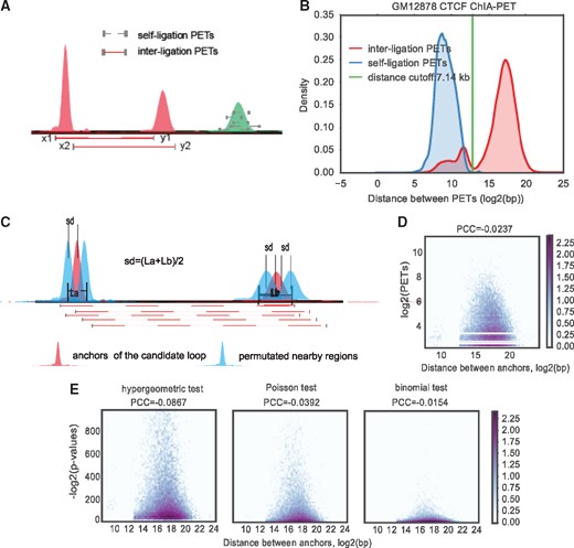
Overview of cLoops. (A) To carry out clustering, each PET is mapped to 2D space as its middle coordinate of left PET mapped to x-axis and right mapped to y-axis. (B) Distance distribution for GM12878 CTCF ChIA-PET PETs in classified inter-ligation and self-ligation clusters. (C) Permutated local background for estimating candidate loops statistical significance. For two anchors of a candidate loop, all combinations of their upstream and downstream five moving windows with size of anchors and step size of the mean length of these two anchors are used as background. The mean distance for all combinations is exactly the same as the interacting loop region. (D) Hexbin plot of detected PETs and distance between loop anchors for CTCF ChIA-PET data. (E) Hexbin plot of estimated P-values using different methods and the distance between loop anchors for CTCF ChIA-PET data

The key parameters used in cLoops are those used to run cDBSCAN, $\mathit{eps}$ and $\mathit{minPts}$⁠. $\mathit{minPts}$ determines the least number of PETs required for a loop, and $\mathit{eps}$ defines the distance for two PETs to be neighbors and this setting is more data dependent. Multiple eps and minPts can be assigned to cLoops to run cDBSCAN clustering multiple times to find merged consensus candidate loops. Empirically determined parameters were used for ChIA-PET [sharp peak, human genome with around 15 million cis-PETs: eps = (500, 1000, 2000), minPts = 5; broad peak, human genome with around 15 million cis-PETs: eps = (1000, 2000, 5000), minPts = 5], HiChIP [human genome with > 100 million cis-PETs: eps = (2500, 5000, 7500, 10 000), minPts = (30, 20)] and Hi-C (human genome with > 200 million cis-PETs) and Trac-looping data [eps = (500, 1000, 2000, 5000), minPts = 5]. In principle, eps could be estimated to the average anchor size of potential loops. Besides, a dataset with low sequencing depth may need large $\mathit{eps}$ to connect scattered PETs. minPts is more related to sequencing depth, as it determines the minimal number of PETs required to support a potential loop. User may try some parameters depending on our pre-set ones, such as keeping the eps same, while changing the minPts according to the ratio of target dataset’s number of cis-PETs to our example dataset’s.

3.3 PLB for estimating significance of candidate loops

For the second step, to test the significance of a candidate loop over the nearby genomic background, a PLB is used (Fig. 2C). Linearly closer anchors in the genome have higher probabilities to capture more PETs linking them due to experimental ligation bias in both ChIA-PET and Hi-C (Paulsen et al., 2014), which needs to be modeled and corrected in loop significance tests. We designed this PLB to save the effort of correcting PET distance bias. For each candidate loop (red peaks), PLBs are defined as all combinations of their upstream and downstream windows (light blue peaks, one upstream and one downstream PLB plotted for the left/right anchor, in cLoops 5 moving windows per side are used to obtain 100 permuted background regions) with the same length as the loop anchors (Fig. 2C). The shifting size for the moving windows is the mean length of these two anchors. Thus, the mean distance of all permutated windows is exactly the same as the candidate loop. Based on the PLB, the commonly used hypergeometric test, Poisson test and binomial test were used together to determine a candidate loop’s statistical significance, a loop is marked significant only if it passes all three statistical tests to increase precision; however, all potential loops clustered from the clustering and filtering step will be output to the result file only with the significant column marked as 0, and users can customize their own cutoffs to obtain loops that meet specific analysis requirements. The details of the mathematical model and cutoff are described in Supplementary Methods.

For cLoops-called loops, due to the density-based clustering method and removal of suspected self-ligation PETs based on distance distributions, PET numbers are actually independent of loop distances. For example, in the CTCF ChIA-PET data, the Pearson correlation coefficient is −0.0237 between PETs numbers and distances between anchors (Fig. 2D). The P-values derived using different statistical tests are also independent of loop distances (Fig. 2E).

3.4 cLoops application to ChIA-PET data

We compared cLoops with three peak-calling based loop-calling tool, ChiaSig (Paulsen et al., 2014), ChIA-PET2 (Li et al., 2016) and Mango (Phanstiel et al., 2015) (Supplementary Table S2) using multiple ChIA-PET datasets (Supplementary Table S1). These three ChIA-PET tools were selected because they are the most frequently used. Running time of these tools is shown in Supplementary Table S3. cLoops is designed with parallel computing, while other tools were not, however, even when cLoops was run with only one CPU it was still much faster than ChiaSig and ChIA-PET2 on the GM12878 CTCF and RAD21 ChIA-PET, the HeLa CTCF ChIA-PET data and K562 H3K4me1 ChIA-PET data (Supplementary Table S3).

Heatmaps and global quality of loops were visualized with mean profile heatmaps of loops (centerNormedAPA heatmaps) and the mean P2M scores, respectively (see Section 2). The centerNormedAPA heatmaps were generated by Juicer APA. In a centerNormedAPA heatmap, loops are aligned in the center, and a high contrast ratio compared to the nearby regions indicates good loop quality. If there are highly interacting regions other than the center in a centerNormedAPA heatmap, it indicates either that there are shifts of loop boundaries or global loop quality is not good.

As a quantitative indicator for enrichment of loops compared to nearby regions, P2M (computed by Juicer APA), is defined as the ratio of the central pixel to the mean of the remaining pixels (Durand et al., 2016). In addition to P2M scores, we also show the global mean P2LL scores (Peak to Lower Left) and the related ZscoreLL scores (suggested by the Juicer documentation) for comparison (Supplementary Fig. S8). A comparison of the loop anchor size distributions indicated that cLoops can identify loops with a larger range in anchor size than other peak identification based algorithms, some of which have a predefined anchor size (Supplementary Fig. S9).

In general, cLoops and Mango outperformed ChiaSig and ChIA-PET2 for all tested ChIA-PET data as indicated by the mean profile heatmaps and the mean P2M scores for ChIA-PET data containing sharp peaks (e.g. CTCF and RAD21) (Supplementary Fig. S2). We noticed that Mango, ChiaSig and ChIA-PET did not work well with histone modification ChIA-PET data, such as with K562 H3K27ac and H3K4me1 datasets. Mango, ChiaSig and ChIA-PET2 identified limited loop numbers, and the loops’ quality was worse compared to cLoops’, as evaluated both by mean profile heatmaps of loops and the mean P2M scores (Fig. 3A, Supplementary Figs S2 and S3B). The CAPA designed by Mango to evaluate quality of loops called from ChIA-PET data through Hi-C data was used to further compare performance. CAPA validated advantages of cLoops and Mango over ChiaSig and ChIA-PET2 (Supplementary Fig. S3A) in enriching for Hi-C interacting signals for ChIA-PET data containing broad peaks (Fig. 3B), and similar performances of cLoops and Mango for ChIA-PET data containing sharp peaks (Supplementary Fig. S3B). Worse performance is partially due to using narrow peak calling model of MACS (Zhang et al., 2008) as default. We showed two randomly selected unique loops called by cLoops from H3K4me1 ChIA-PET data (Fig. 3C) and H3K27ac ChIA-PET data (Fig. 3D) as examples to illustrate cLoops’ ability to detect reliable loops that could be observed from the visualization of raw PETs which are missed by other tools. Moreover, Mango estimated P-values showed higher dependence on anchors’ distance, showing higher significance for closer anchors, which suggests insufficient correction for the experimental bias (Supplementary Fig. S3C).

Fig. 3.

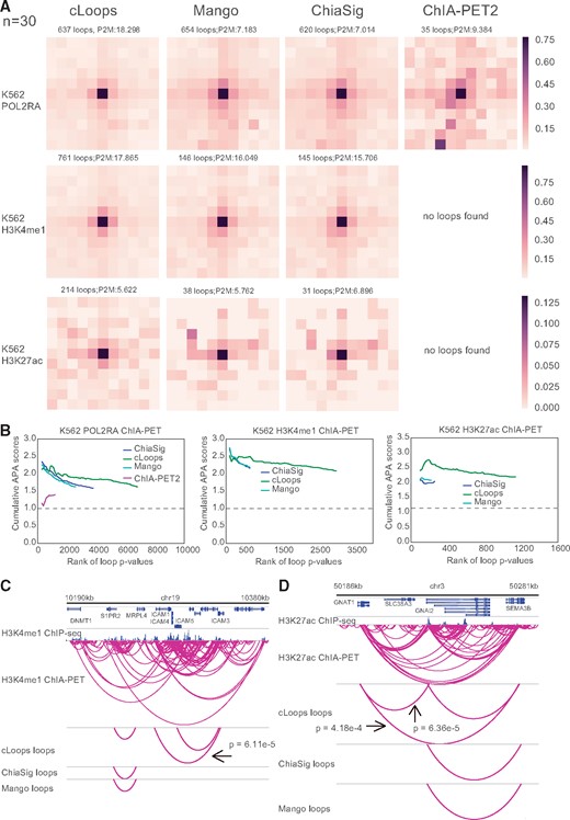
cLoops applied to ChIA-PET data and comparison with other tools. (A) centerNormedAPA heatmaps from Juicer (Durand et al., 2016) APA were shown for loops obtained by cLoops from K562 POLR2A, H3K27ac and H3K4me1 ChIA-PET data. The number of loops and P2M score from whole genome-wide analysis were annotated at head of each dataset heatmap. The P2M score is the mean of all P2M values, which indicate the enrichment of loops compared to nearby regions. In the Juicer APA analysis, n was set to 30 (default parameter) to analyze loops with anchor distance ≥ 150 kb. More comparisons for distance filtered loops are shown in Supplementary Figure S2. (B) CAPA for evaluating the qualities of loops called from ChIA-PET data using Hi-C data. Higher scores mean the loops are better supported by Hi-C (APA score > 1.0). (C, D) Example of unique loops detected by cLoops for H3K4me1 (C) and H3K27ac (D) ChIA-PET data, labeled p values in figure are the maximal Bonferroni corrected p values from poisson, binomial and hypergeometric test for the loops

3.5 cLoops application to Hi-C data

We compared cLoops with five Hi-C loop-calling tools recently evaluated in a tool-performance comparison study (Forcato et al., 2017), namely diffHic (Lun and Smyth, 2015), Fit-Hi-C (Ay et al., 2014), GOTHiC (Mifsud et al., 2017), GPU-version HiCCUPS (Durand et al., 2016) and HOMER (Heinz et al., 2010) (Supplementary Table S2), using the high-resolution deep sequencing data from GM12878 and K562 Hi-C data (Supplementary Table S1). CPU-version HiCCUPS was not included in the comparison because it ignores distant loops detection to achieve acceptable speed which makes it inherently worse than corresponding GPU version (Supplementary Fig. S1A). In the meantime, cLoops does not require a specific setting for calling loops as it already takes the distance into consideration by using local background for significance evaluation. To compare performance on the same hardware system, we run all programs in same PC system (Supplementary Information) with equivalent pre-processing using HiC-Pro. We did not compare HIPPIE (Hwang et al., 2015) for following reasons: (i) HIPPIE requires Sun Grid Engine system but to compare tools based on equivalent systems we could only access a PC system with GPUs. (ii) HIPPIE require its own pre-processing pipeline which uses STAR (Dobin et al., 2013) for mapping. (iii) HIPPIE did not show unique advantages for calling loops in the comparison study (Forcato et al., 2017). Parameters and loops selections were mostly set according to those used in a previous comparison study (Forcato et al., 2017) (Supplementary Table S2). Raw FASTQ data was first processed by HiC-Pro and the required input files for each tool were converted from HiC-Pro output files (Supplementary Methods). The runtimes of these tools are available in Supplementary Table S4.

For both GM12878 and K562 Hi-C data, a region on chromosome 21 (36 000–39 500 kb) contained six obvious, conserved, visibly salient loops in the 5 kb resolution heatmaps (5 kb resolution was chosen for visualization in Juicebox to get clear view of loops and 5 kb is the default high-resolution setting for a .hic file visualized in Juicebox), designated as ‘a’, ‘b’, ‘c’, ‘d’, ‘e’, ‘f’ (note that there are actually two loops at the ‘e’ region if further zoomed-in) (Supplementary Fig. S10A and B). We compared loops detected by different tools in this example region for both Hi-C and following HiChIP data. Generally, cLoops and HiCCUPS outperformed other tools in detecting most of the visible loops and not reporting probable false-positives located near the heatmap diagonal for both GM12878 and K562 data (Supplementary Fig. S10A and B, Supplementary Fig. S5A). More examples of visible loop comparisons are shown in Supplementary Figure S6. The mean loop profile heatmaps and mean P2M scores indicated that the majority of loops detected by diffHic, Fit-Hi-C, GOTHiC and HOMER are located very near to the diagonal line and have no enriched interaction signals compared to nearby regions. The distribution of distances between loop anchors also supported this conclusion, as HOMER and GOTHiC tended to identify closer loops which represented distance dependency (Supplementary Fig. S4E). The mean profile heatmaps showed cLoops had higher enrichment of interacting signals of loops compared to nearby regions (Supplementary Fig. S10A and B, Supplementary Fig. S5A). We manually marked visually reliable loops spotted on human chr21 (Supplementary Tables S7 and S8), used them as true positives to plot precision-recall curve for all the tools, and found that cLoops also achieved better performance than other tools (Supplementary Fig. S4G and H).

Fig. 4.

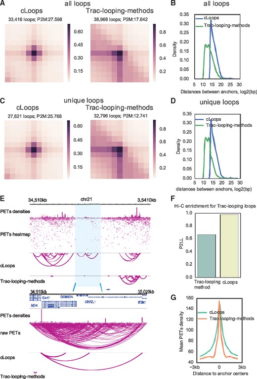
cLoops applied to Trac-looping data compared to the Trac-looping-methods. (A) Mean profile heatmaps of all loops called cLoops and the Trac-looping-method. Mapped PETs of Trac-looping data for the resting CD4 cell in BEDPE files and the Trac-looping-methods called were obtained from GSE87253. (B) Distribution of distances between loop anchors for all loops. (C) Mean profile heatmaps of unique loops called by cLoops and the Trac-looping-methods. (D) Distribution of distances between loop anchors for unique loops. (E) Randomly selected examples for cLoops and Trac-looping-methods called loops. (F) APA for evaluating the qualities of loops called from Trac-looping data using Hi-C data. The P2LL (peak to lower left, suggested by Juicer) was used to show enrichment of Hi-C signal on Trac-looping loop regions. (G) Mean Trac-looping PETs densities on loop anchors

For independent confirmation, the higher overlap of cLoops and HiCCUPS called GM12878 Hi-C loops with cLoops called or Mango called CTCF and RAD21 ChIA-PET loops (Supplementary Fig. 4A and B) and cLoops called or HiCCUPS called HiChIP loops (Supplementary Fig. S4C) supported the robustness of performance of cLoops and HiCCUPS over other tools. That is, higher mean density of CTCF, RAD21 and SMC3 ChIP-seq binding signals on anchors called by cLoops and HiCCUPS strongly supported their higher accuracy and comparatively better performance. Moreover, we also observed two distinct advantages of cLoops compared to all other tools: (i) for called loops, the PET numbers were less dependent on distance between anchors (Supplementary Fig. S4D) and (ii) cLoops can better detect more distant loops (Supplementary Fig. S4E).

HiCCUPS is mainly based on comparing observed values to expected values for every pixel (where pixel size depends on the pre-defined resolution for contact matrix), and then, determining the significance for the pixel using a modified Benjamini-Hochberg FDR control procedure (so called ‘$\lambda$-chunking’), with additional filters for local neighborhoods. Then, the loops are clustered from significant pixels. The concept of the HiCCUPS algorithm is quite different from cLoops; the setting of Hi-C specific ‘$\lambda$-chunking’ and the additional filters may limit HiCCUPS to few types of 3D-genomic data, and the time-consuming pixel level computing is also limited to an inside loops distance cutoff (≤2 MB), while cLoops does not. Overall, cLoops’ loops were better supported by ChIA-PET and HiChIP data overlap in GM12878 and showed less bias against distant loops.

3.6 cLoops application to deep-sequencing HiChIP data

Although Fit-Hi-C and Mango were used for calling loops in their original HiChIP method paper (Mumbach et al., 2016), only HiCCUPS called loops using merged PETs from biological and technical replicates were provided as Supplementary Data, so we first compared cLoops to HiCCUPS using the merged GM12878 cohesin HiChIP data.

cLoops obtained similar numbers of loops as HiCCUPS for the GM12878 cohesin HiChIP data on the example chromosome 21 region mentioned above in the Hi-C comparisons (Supplementary Fig. S10), where cLoops detected all six visible loops (Supplementary Fig. S11A). HiCCUPS did not detect loop ‘f’ despite detecting the ‘f’ loop in Hi-C data (Supplementary Fig. S11A). The mean loops profile heatmaps indicated HiCCUPS may detect more loops close to the heatmap diagonal line (Supplementary Fig. S11B and C). We validated this by showing distance between anchors for all loops (Supplementary Fig. S11F), unique loops’ mean profile heatmap for cLoops and HiCCUPS (Supplementary Fig. S11G) and distance between anchors for unique loops (Supplementary Fig. S11I), which altogether showed cLoops can detect more distant loops and loops called by cLoops had higher signal enrichment. Furthermore, loops called by cLoops are better supported by both ChIA-PET loops and Hi-C loops for all called loops (Supplementary Fig. S11E and Supplementary Fig. S7A), and for the unique loops (Supplementary Fig. S11H and Supplementary Fig. S7B). Moreover, the loop anchors called by cLoops have higher CTCF, RAD21 and SMC3 ChIP-seq tag densities than those of HiCCUPS (Supplementary Fig. S11D).

3.7 cLoops application with low-depth sequencing HiChIP data

With the capture enrichment process, HiChIP could in principle reveal enriched loops with under-sequenced PETs compared to Hi-C. Therefore, we wondered whether cLoops’ performance is still relatively good in this situation. We compared cLoops with the Hi-C loop-calling tools compared above and hichipper (Lareau and Aryee, 2018) (Supplementary Table S2) using the two technical replicates of biological replicate one from the cohesin GM12878 HiChIP data. Running time of these tools was shown in Supplementary Table S5. Even use only one CPU, cLoops was faster than HOMER, hichipper, Fit-Hi-C and GOTHiC.

The performances of each tool were assessed in a similar way as for Hi-C data above. For the low-depth sequenced HiChIP data, in summary, (i) cLoops, HiCCUPS, HOMER and hichipper can obtain similar visible loops as shown in the example region (Supplementary Fig. S12A), detecting majority of the four example loops (‘a’, ‘b’, ‘c’, ‘d’) on the heatmaps for both replicates, and not detecting artificial interaction signals close to diagonal line. Also, the mean profile heatmaps for all loops from all four tools showed enrichment over nearby regions, while loops from diffHic and GOTHiC showed obvious patterns close to the diagonal line (Supplementary Fig. S12B) Loops called by cLoops, HiCCUPS and HOMER were consistent with CTCF ChIA-PET loops (Supplementary Fig. S7C), RAD21 ChIA-PET loops (Supplementary Fig. S7D) and Hi-C loops (Supplementary Fig. S7E), as measured by the Jaccard index. (iii) The detected PET numbers in loops called by cLoops and HiCCUPS are far less dependent on distance between anchors than in loops called by other tools (Supplementary Fig. S7F). The distance dependence is especially high for HOMER, hichipper and Fit-Hi-C. (iv) cLoops, HiCCUPS and Fit-Hi-C could detect more distant loops compared to others (Supplementary Fig. S7G). Notably, cLoops does not need additional control parameters like –L and –U in Fit-Hi-C to detect distant loops. (v) HiCCUPS and cLoops had the highest Jaccard Index of overlapping loops between technical replicates, except for GOTHiC, as it appeared to call too many loops (e.g. in the example region GOTHiC called loops at nearly all positions), whereas hichipper showed the lowest Jaccard Index, indicating the peak-based strategy might be biased by errors in peak calling (Supplementary Fig. S7H). (vi) The anchors of loops detected by cLoops, HOMER and hichipper are better supported by the CTCF, RAD21 and SMC3 ChIP-seq data (Supplementary Fig. S7I). Due to the first pre-customized peak-calling step of hichipper, the higher enrichment of ChIP signal on hichipper anchors is expected by design. (vii) Again, cLoops does not need GPU like HiCCUPS.

3.8 cLoops application to trac-looping data

We further demonstrated the generality of cLoops for calling accurate loops using the recently published Trac-looping data (Lai et al., 2018). The advantages of cLoops over the Trac-looping-methods are shown by the following: (i) Globally, loops called by cLoops were more enriched for the Trac-looping PETs compared to nearby regions (Fig. 4A). (ii) cLoops detected much more distant loops (Fig. 4B). (iii) The loops uniquely detected by cLoops were much more enriched for interacting signals (Fig. 4C) and most of the uniquely detected loops of cLoops are more distant (Fig. 4D). A randomly selected example shows three distant loops uniquely detected by cLoops as linking the significant interactions between promoters while the Trac-looping-methods detected a very close loop nearby (Fig. 4E). (iv) Hi-C signals on the Trac-looping loops also show higher enrichment of cLoops called loops compared to the Trac-looping-methods (Fig. 4F). Even though there was no peak-calling step in cLoops, the PETs density on cLoops called loop anchors were as high as that of the Trac-looping-methods (Fig. 4G).

4 Discussion

In summary, we report cLoops as a new loop-calling tool based on an improved clustering algorithm, cDBSCAN and PLB. We first showed the cDBSCAN clustering algorithm drastically improved speed on both simulated data and real CTCF ChIA-PET data compared to the original DBSCAN algorithm. From multiple re-sampling 3D genomic data, cDBSCAN shows near O(N) algorithmic complexity in current data scale. cLoops determines the significance of loop calling by a permuted, instead of model-based, local background. These two features make cLoops applicable to ChIA-PET, HiChIP, Hi-C and Trac-looping data, other 3C-based chromatin interaction data, and yet-to-be-developed 3D mapping technologies.

One limitation for the comparison carried in this study and maybe others is that we and others did not have a compiled gold positive standard and negative standard loops for all available data to conclude which tool is truly the best in loop calling, considering the accuracy and false discovery rate as the direct evidence, more experimentally verified or properly generated simulation data is needed for the tools developing community. As current cLoops is coded in python, when used on ChIA-PET, HiChIP and Trac-looping data, it can be relatively time-consuming for loop-calling with deeply sequenced Hi-C data (such as more than 200 million raw PETs used in this study), which need further algorithm improvement. Although current version of cLoops is implemented with parallel computing, the running time could be dramatically reduced by using more CPUs if the RAM is enough for the servers, re-writing only core parts of cLoops such as cDBSCAN with lower level programming language (such as Cython or C) could boost the power of cLoops for deeply sequenced data.

Author contributions

Y.C. and J.D.J.H. designed the project; Y.C. and X.C. implemented the cDBSCAN algorithm; Y.C. and D.A. implemented the local permutated significance test model. Y.C., Z.C. and D.A. performed comparison analysis. All authors contributed to data analysis, interpretation and wrote the paper.

Funding

This work was supported by grants from National Natural Science Foundation of China [91749205, 91329302 and 31210103916], China Ministry of Science and Technology [2015CB964803 and 2016YFE0108700] and Chinese Academy of Sciences [XDA01010303 and YZ201243] and Max Planck fellowship to J.D.J.H.

Conflict of Interest: none declared.

Author notes

Yaqiang Cao and Zhaoxiong Chen wish it to be known that, in their opinion, the first four authors should be regarded as Joint First Authors.