phyLoSTM: a novel deep learning model on disease prediction from longitudinal microbiome data

Abstract

Motivation

Research shows that human microbiome is highly dynamic on longitudinal timescales, changing dynamically with diet, or due to medical interventions. In this article, we propose a novel deep learning framework ‘phyLoSTM’, using a combination of Convolutional Neural Networks and Long Short Term Memory Networks (LSTM) for feature extraction and analysis of temporal dependency in longitudinal microbiome sequencing data along with host’s environmental factors for disease prediction. Additional novelty in terms of handling variable timepoints in subjects through LSTMs, as well as, weight balancing between imbalanced cases and controls is proposed.

Results

We simulated 100 datasets across multiple time points for model testing. To demonstrate the model’s effectiveness, we also implemented this novel method into two real longitudinal human microbiome studies: (i) DIABIMMUNE three country cohort with food allergy outcomes (Milk, Egg, Peanut and Overall) and (ii) DiGiulio study with preterm delivery as outcome. Extensive analysis and comparison of our approach yields encouraging performance with an AUC of 0.897 (increased by 5%) on simulated studies and AUCs of 0.762 (increased by 19%) and 0.713 (increased by 8%) on the two real longitudinal microbiome studies respectively, as compared to the next best performing method, Random Forest. The proposed methodology improves predictive accuracy on longitudinal human microbiome studies containing spatially correlated data, and evaluates the change of microbiome composition contributing to outcome prediction.

Availability and implementation

https://github.com/divya031090/phyLoSTM.

Supplementary information

Supplementary data are available at Bioinformatics online.

1 Introduction

Microbiome inherently is dynamic in nature, attributing to the presence of interactions among microbes, microbes and the host and with the environment. Researchers have shown that the microbiome can be altered over time, either transiently or long term, by infections or medical interventions such as antibiotics (Faust et al., 2015; Gilbert et al., 2018; Gonzalez et al., 2012). Recent advances in high-throughput experimental technologies are enabling researchers to measure dynamic behaviors of the microbiota at a large scale (Bäckhed et al., 2015; Chen and Xu, 2020; Gerber, 2014). Comprehensive analyses of the microbiota over time, provide insights into essential questions about microbiome dynamics, for example, how microbiome composition changes through infection/antibiotics and do changes in the microbiome cause or increase susceptibility and risk of certain diseases. Longitudinal data provides more information than single time point data because temporal information creates an inherent ordering in microbiome samples, and thereby they exhibit statistical dependencies that are a function of time (Caporaso et al., 2011; Kostic et al., 2015; Morris et al., 2016). These features enable discovery of rich information about microbial data, including short and long-term trends. Therefore, it is imperative to analyze longitudinal microbiome studies for risk prediction. However, major challenge with longitudinal microbiome data is the presence of uneven number of timepoints along the longitudinal timeline of different subjects (Ridenhour et al., 2017), making it necessary for the use of appropriate computational techniques to address this issue.

Deep learning has proven to be an efficient methodology to derive knowledge from the vast amount of data available from biomedical studies (LaPierre et al., 2019; Oh and Zhang, 2020). The existing studies explore long-term dependencies/trends by regressing a series of observations on time (Wei, 2006). A few studies also analyzed longitudinal microbiome data using Hidden Markov Models (HMM) (Rabiner and Juang, 1986). However, the performance of HMMs is highly impacted by the difference in the number of timepoints in microbiome data for each subject, hence, HMMs require an additional alignment of the longitudinal taxonomic profiles for each subject (Stein et al., 2013). Lugo-Martinez et al. (2019) also proposed taxonomic profile alignments coupled with dynamic Bayesian networks for analyzing longitudinal microbiome data. To mitigate the issues arising due to uneven time points in longitudinal microbiome analysis, we propose novel Long Short-Term Memory (LSTM) networks (Hochreiter and Schmidhuber, 1997) to study the temporal information and dynamic behaviors in microbiomes. LSTMs are widely popular in time series prediction tasks such as, sentence completion, speech recognition, etc. (Graves and Schmidhuber, 2005; Schmidhuber et al., 2002). Since there can be lags of unknown duration between important events in a time series, therefore, relative insensitivity to gap length and dealing with vanishing gradient issue is an advantage of LSTM over Recurrent Neural Networks (Graves et al., 2013), Hidden Markov models and other sequential learning methods in numerous applications (Chung et al., 2015). A recent study (Metwally et al., 2019) utilized the LSTMs for analyzing longitudinal microbiome data, however, it only proposed basic feature extraction technique from Operational Taxonomic Unit (OTU) data using autoencoders and reports low prediction level accuracy, infeasible for clinical utilization.

To address these challenges, in this article, we explore the abilities of longitudinal microbiome data to predict risk of disease using a novel two-step approach combining the power of Convolutional Neural Networks (LeCun et al., 1998) for automatic feature extraction and LSTMs for temporal feature understanding (Sainath et al., 2015; Shi et al., 2015). A broad overview of our goal is illustrated in Figure 1. Currently, as per our knowledge, there is no systematic methodology evaluation to assess longitudinal change in microbiome along with the host’s clinical factors for disease/risk prediction. We aim to explore the complex interactions within the microbiome and between taxa and clinical factors (e.g. demographics, age etc.) (Knights et al., 2014) and also capture temporal information to understand the dynamic changes in microbiomes (Lugo-Martinez et al., 2019). We hypothesize that adding the information from past microbiome profiles increases the predictive power of the microbiome sequencing data in comparison to training a model with microbiome data at each timepoint independently. Our framework is empowered by the LSTM’s capacity for making robust strategies to extract abstract non-linear features without the explicit need to align the longitudinal taxonomic data for prediction of the clinical outcome (Hochreiter et al., 2007).

Fig. 1.

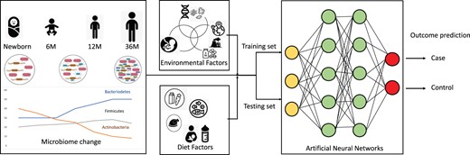
Broad overview of objective on risk prediction using longitudinal microbiome profiles along with environmental and diet factors

We propose a novel computational algorithm and analytic pipeline, wherein, the input to the feature selection/extraction module is a vector representing a normalized taxonomic profile (OTUs) of a subject’s microbial sample along with the associated clinical factors. Our major contribution is in providing a comprehensive novel pipeline for better feature extraction from microbiome data at various time points and finally to predict disease/risk while taking in account the temporal changes in the microbiome, thereby increasing prediction efficiency. Three key points of novelty are: (i) pre-processing the microbiome data to exhibit spatial taxonomic similarity, so that the CNN can extract the OTU data features efficiently (Sharma et al., 2020). The selected or extracted features are then passed to the LSTM module to learn temporal dependency between sequence profiles, (ii) weight balancing of binary classes in the LSTM learning to deal with class imbalance, mitigating scenarios where number of cases are usually less in comparison to the controls, causing the neural network learning to be biased and inaccurate, (iii) robust testing demonstrated by two real studies, one of which contains four different outcomes and another contains microbiome data from multiple body sites, validating the generalizability of our approach.

2 Materials and methods

2.1 Proposed framework

We propose phyLoSTM, a two-step modeling for feature extraction and thereafter learning temporal dependencies in the longitudinal microbiome sequencing data. We achieve this through a combination of Convolutional Neural Networks (CNNs) and Long Short Term Memory networks (LSTMs). The proposed two-step framework is shown in Figure 2a. The taxonomic profile in the form of input OTU vector is provided to the CNN module for feature extraction as shown in Figure 2b. The CNN module incorporates the inherent phylogenetic relationship in the OTU data before providing it as an input to the neural network model. Where firstly the OTU data is rearranged based on the correlation in the OTUs sharing the same parent phylum. In the second step, an LSTM module as shown in Figure 2c is invoked, which learns the temporal dependencies in the longitudinal microbiome profiles, through learning a new state of interdependent temporal profile based on previous state. Details of the two-step modeling approach are provided in the next subsections.

Fig. 2.

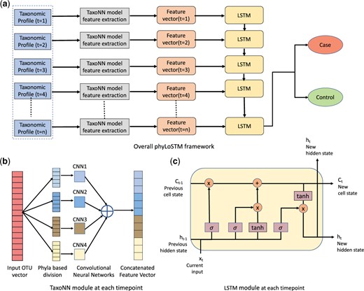
Overall Framework for longitudinal microbiome analysis for disease prediction. (a) Proposed ’phyLoSTM’ framework. (b) Stratified CNN (taxoNN) module for feature extraction. (c) LSTM network module to learn temporal dependencies

2.1.1 Feature extraction through stratified CNN

To extract features efficiently from OTU data, we propose a CNN network suited for the OTU data structure. Let there be ‘n’ subjects in the whole study, with repeated measures across ‘k’ time points. The OTU data for i^th subject (where $i\in$ n), is presented in a 1-D vector format to the network, as, $OT{U}_{i^{th}s\mathit{ubject}}=\{o_1,o_2\mathrm{\dots .},o_N\}$⁠, where N is the total number of OTUs in a subject. In place of using unstructured OTU data, without looking into spatial relationships in the data, we use a stratified approach, where we first divide OTU data into phyla groups. The phyla groups are chosen based on phylum containing majority of OTUs. Further, ensemble of convolutional neural networks is applied to each phyla group to extract features. Herein, two aspects of OTU data structure are explored i.e. the taxonomy, as well as, the correlation between OTUs to create similarity between adjacent OTUs. Spearman rank coefficient matrix of the OTUs within each phyla cluster is used to capture similarity in adjacent OTUs. Each row of the Spearman rank coefficient matrix(p × p matrix for p OTUs in a cluster) is reduced to a cumulative correlation coefficient, using the formula:

$${\rho }_{OT{U}_{ro{w}_j}}=\sqrt[p]{\left|{\rho }_{OT{U}_{j1}}\right|·\left|{\rho }_{OT{U}_{j2}}\right|\mathrm{\dots .}·\left|{\rho }_{OT{U}_{jp}}\right|}$$

(1)

for $j\in [1,p].$

Further, each of these cumulative coefficients are arranged in a decreasing order forming a sorted vector ${\mathrm{P}}_{\mathit{OTU}}^{*}$ using the formula:

$${\mathrm{P}}_{\mathit{OTU}}^{*}=\{{\rho }_{OT{U}_{\mathit{row}5}},{\rho }_{OT{U}_{\mathit{row}3}}\mathrm{\dots ..},{\rho }_{OT{U}_{ro{w}_p}}\}$$

(2)

Subsequently, the heatmap obtained by the correlations in the OTU data is re-ordered based on the decreasing order of the cumulative correlation coefficients. Through this ordering, the correlation structure between the OTUs is used to establish a similarity in the neighbouring OTUs before being provided to the CNN model. This variation of CNN modeling is named as taxoNN_corr (Sharma et al., 2020). The CNN model is defined using two 1-Dimensional convolutional layers, each followed by a pooling layer. The CNN is applied individually to each phyla group and features are extracted from the major phyla groups. Next, ensemble learning (Hansen and Salamon, 1990) is used, where features from each group are combined. The flattened feature vectors obtained from each group are merged via concatenation to make one very long vector that is then interpreted and sent to the LSTM module for learning the temporal dependency.

2.1.2 Long Short Term Memory Networks (LSTM)

LSTM learn time-based dependencies in data. A common LSTM unit is composed of a cell, an input gate, an output gate and a forget gate. The LSTM has ability to remove or add information to the cell state (C_t), carefully regulated by structures called gates. The sigmoid layer decides on preserving significant aspects of the input through observing the previous hidden layer’s output, $h_{t-1}$ and current input x_t, and outputs a number between 0 and 1 stored in f_t.

$$f_t=\sigma (W_f.[h_{t-1},x_t]+b_f)$$

(3)

In the next step, another sigmoid layer decides which values to update. Further, a tanh layer creates a vector of new candidate values $C_t^{*}$⁠, that need to be added to the cell state. In the next step, combination of these two is conducted to create an update to the state.

$$i_t=\sigma (W_i.[h_{t-1},x_t]+b_i)$$

(4)

 

$$C_t^{*}=\tanh (W_C.[h_{t-1},x_t]+b_C)$$

(5)

The old cell state $C_{t-1}$ is multiplied by f_t (obtained in Equation 3), to keep/forget essential data during passing of information from one time point to another. Then $i_t*C_t^{*}$ are added forming the new candidate value, scaled by i_t, which is the factor by which each state value is updated.

$$C_t=f_t*C_{t-1}+i_t*C_t^{*}$$

(6)

Finally, the output is based on the filtered version of the cell state, wherein, a sigmoid layer decides what parts of the cell state to output. Then, the cell state is passed through tanh (to push the values to be between -1 and 1) and multiplied by the output of the sigmoid gate, to only output essential parts of the data.

$$o_t=\sigma (W_o.[h_{t-1},x_t]+b_o)$$

(7)

 

$$h_t=o_t*\tanh (C_t)$$

(8)

The weights and biases used in above equations are, W_f, b_f: Forget gate weight and bias, W_i, b_i: Input gate weight and bias, W_C, b_C: Candidate cell state weight and bias and W_o, b_o: Output gate weight and bias. Through the series of steps as listed through Equations 3–8, the new cell state, as well as, the hidden state from the LSTM network are generated at a given single timepoint. This ensures preserving information from the previous timepoint and forwarding to the succeeding timepoint, to learn the temporal relationship.

Finally, the flattened vectors obtained are vectorized into a very long vector that is then interpreted and sent to final classification layer that has a binary node with a softmax activation:

$$V_t=W_v*h_t+b_t$$

(9)

 

$$y_t=\mathit{softmax}(V_t)$$

(10)

where W_v, b_v are the weight and bias associated with the Softmax layer.

Handling variable time points in data

Padding and masking operations are applied by the LSTM to handle the variability in length of data for each subject at various timepoints (Neubig et al., 2017). Firstly, inputs are sorted by subjects’ containing the longest sequence first. Subsequently, all the other sequences are made of the same length by padding to largest sequence length in the batch. Further masking is done of the padded sequence, to make sure LSTM does not see padded items. All masked values are ignored and the output and state for those time steps are copied over from the last non-masked state. The error of prediction is calculated and back-propagated through the system to improve the learning. This padding and masking in LSTMs helps in dealing with uneven number of timepoints along the subjects’ longitudinal timeline.

Weighted cross entropy handling data imbalance

The microbiome data often suffers with the issue of imbalance in the number of cases and controls, where samples in cases are usually less in number than the controls (Baxter et al., 2016; Goodrich et al., 2014). Under such situation, the learning of the neural network can be improper. The main reason being, the network does not get optimized results for the imbalanced class in real time as the model/algorithm never gets sufficient look at the underlying class. Therefore, to handle the imbalance, we propose a weight balancing approach in the CNN network by giving higher weights in the loss function, to the class which has less samples (i.e. the cases in our scenario).

The loss function we use in our LSTM module is Cross-entropy which is defined as:

$$\mathit{Cross}\hspace{0.17em}\mathit{Entropy}=-\mathit{ylog}(p)-(1-y)\mathit{log}(1-p)$$

(11)

where y is the class binary indicator (0 or 1) (refer equation 10) and P is predicted probability for instance belonging to class 1. To incorporate the weights of two classes (0 and 1) into the cross entropy, one can define a weighted cross entropy:

$$\mathit{Weighted}\hspace{0.17em}\mathit{Cross}\hspace{0.17em}\mathit{Entropy}=-w_o*\mathit{ylog}(p)-w_1*(1-y)\mathit{log}(1-p)$$

(12)

where w₀ and w₁ are the weights for class 1 and 0, respectively.

The weight to the classes can be given by multiplying the loss of each example by a certain factor (weight) depending on their class (higher weight to class with less samples). Instead of spending time and resources trying to collect more samples for the minority class, we can try to use weight balancing to make all classes contribute equally to the loss. Such an approach of weight balancing is more efficient than using oversampling based on replication of samples in cases and controls. Replication creates a copy of samples and makes the neural network learning biased and leads to over-fitting to the training data making learning inaccurate.

2.2 Datasets

2.2.1 Simulated studies

We designed simulation studies based on the microbiome data based on the DIABIMMUNE project’s three country cohort (Vatanen et al., 2016). Our simulated datasets were created by using 785 repeated samples provided in the DIABIMMUNE study data. Each subject contained 534 OTUs. The OTUs in this simulated dataset were categorized into taxonomy levels with 12 phyla. The three dominant bacterial phyla in terms of the number of OTUs were Firmicutes, Proteobacteria and Bacteroidetes.

We used this data to create a population with 100 000 samples at six time points, ensuring a sample from a timepoint is simulated only by using data available for that particular timepoint. Instead of a simple replication we added noise to each OTU using a normally distributed function with mean equal to a random number in the range $[1\times {10}^{-6},2\times {10}^{-6}]$ and standard deviation of ${10}^{-6}$ to create new samples. While doing so we ensured that we preserve the zeroes and also considered that the relative abundance is equal to one, by adding and subtracting the noise term in equal proportion in each OTU set, keeping the zeroes. We then generated the disease status (y = 1 for case; y = 0 for control) using the formula:

$$p(y=1)=\frac{\hspace{0.17em}\text{exp}(\alpha +\sum _{i=1}^{32}{\beta }_i·OT{U}_i+\sum _{i=1}^2\sum _{j=i+1}^3{\beta }_{ij}·OT{U}_i·OT{U}_j+\gamma ·t)}{1+\text{exp}(\alpha +\sum _{i=1}^{32}{\beta }_i·OT{U}_i+\sum _{i=1}^2\sum _{j=i+1}^3{\beta }_{ij}·OT{U}_i·OT{U}_j+\gamma ·t)}$$

(13)

where β_i were the regression coefficients associated with OTUs, α was the base prevalence, β_ij were the regression coefficients for the pairwise interaction terms, γ was the regression coefficient for the time variable (t), y was the outcome variable and $p(y=1)$ was the probability of the outcome variable to be 1, i.e. disease status positive. In general, the causal OTUs that are potentially associated with risk of disease, in a microbiome dataset are unknown and their number can range from zero to a very large value. Carefully choosing the number of these causal OTUs during simulating data, thus, becomes a challenge. Therefore, based on a trade-off between the model performance upon analysis with various number of causal OTUs (Supplementary Table S1) and the realistic estimation of OTUs that are potentially associated with risk of disease in a real microbiome dataset, we selected 32 OTUs randomly as the OTUs that were potentially associated with risk of disease, also ensuring that all clusters contribute to these causal OTUs. We set the value of α as -2.5, β_i in 1st cluster ranging from [1,1.5], 2nd cluster ranging from [1,2], 3rd cluster ranging from [1.5,2] and 4th cluster [0.5,1]. Interaction terms were added to introduce non-linearity in the data. Out of the 32 causal OTUs potentially associated with risk of disease, 3 OTUs were randomly picked and three pairwise interactions between them were generated (as shown in Equation 13), where β_ij was taken as [1,1.5,2]. For the time covariate in the equation, γ was taken to be 0.1. In this way, we generated 2000 samples as cases and 98 000 as controls from the 100 000 samples.

Considering the drop off nature of the longitudinal measures over time, in the 1st timepoint, we considered, 500 controls and 300 cases, which reduced to 450 controls and 250 cases in the 2nd timepoint, 400 controls and 200 cases in the 3rd timepoint, 350 controls and 150 cases in the 4th timepoint, 300 controls and 100 cases in the 5th timepoint and for the final 6th timepoint we had, 250 controls and 50 cases, from the simulated 98 000 control and 2000 case samples. 100 replication simulation datasets were generated following the same strategy.

The phyla-based stratification on the OTUs in the simulated dataset was done in the following manner: for 534 OTUs, after phyla-based stratification, 1st cluster contained 257 OTUs, 2nd contained 106 OTUs, 3rd contained 88 OTUs and 4th contained 83 OTUs. Each cluster was provided as an input to an individual CNN to understand the relationships between OTUs inside each phyla and later the extracted features were used for passing on to the LSTM network for temporal-based predictions.

2.2.2 Real studies

To assess the prediction power of phyLoSTM on predicting disease risk using longitudinal microbiome data, we implemented our algorithm directly on the DIABIMMUNE three country cohort (Vatanen et al., 2016) and a case-control study for preterm delivery conducted by DiGiulio et al. (DiGiulio et al., 2015).

DIABIMMUNE three country cohort: In this real study, subjects were infants, recruited from three countries having substantial differences of incidence of type 1 diabetes (T1D) and allergies: 71 infants from Finland, 71 infants from Estonia and 70 infants from Russia were recruited. Infants from each country were selected on the basis of similar HLA risk (predisposition to T1D) and matching gender. For each infant, three years of monthly stool samples, laboratory assays and questionnaires regarding breastfeeding, diet, allergies, infections, family history, use of drugs and clinical examinations were collected. In order to study the gut microbiome of these infants, a total of 785 stool samples using whole-genome shotgun sequencing were obtained. This study contains metagenomic data for 212 unique infants with repeated measures making the total count of subject samples to 785. We have various allergy status serving as the outcome in this real study. For some of the subjects, outcomes were not available in the study, hence only 732 samples with outcome information were selected for the analysis. We selected three allergy outcomes for our final analysis, milk allergy, egg allergy and peanut allergy, all containing 534 OTUs at the species level in the kingdom ‘Bacteria’. We also combined all these allergy outcomes to constitute an ‘overall allergy’ variable.

In the study, Proteobacteria, Bacteriodetes and Firmicutes emerged as the phyla with majority of OTUs, leading to form three major clusters for our phyLoSTM. Supplementary Table S2 gives more details about the OTUs in each cluster in the study. We included all environmental variables that were collected in the study namely, age at collection of samples, delivery mode, gender, ethnicity, breast feeding status to predict disease status to ensure our performance evaluation does not miss any potential associated environmental variables to study outcome. Details of the distribution of these variables are provided in Supplementary Table S3. We divided the subjects into six timepoints for our longitudinal analysis. These time points were interpreted from the sample collection time provided in the study in months. We then defined each timepoint (T1 to T6) at 6, 12 18, 24, 30 and 36 months of the sample collection. The box-plots containing relative abundance percentages of OTUs in each phylum of the study at six different time points measured every six months for infants uptil the age of three, are presented in Supplementary Figure S7. It is to be noted, that certain subjects had missing data for some time points, which was dealt in the LSTM network using padding and masking. 110 samples were present at timepoint T1, 197 samples at timepoint T2, 220 samples at timepoint T3, 161 samples at timepoint T4, 54 samples at timepoint T5 and 43 samples were present in the study at timepoint T6. Further details of distribution of cases and controls at each time point is provided in Supplementary Table S4.

DiGiulio case–control study: This is a case-control study comprising of 40 pregnant women, 11 of whom delivered preterm serving as the outcome. Overall, in this study there are 3767 samples with 1420 microbial taxa from four body sites: vagina, distal gut, saliva and tooth/gum. In addition to bacterial taxonomic composition, clinical and demographic attributes included in the dataset are, gestational or post-partum day when sample was collected, race and ethnicity. Details of the distribution of these variables are provided in Supplementary Table S6. In the study Proteobacteria, Bacteriodetes and Firmicutes emerged as the phyla with majority of OTUs, leading to form three major clusters for phyLoSTM. In this study, we divided the subjects into four timepoints for longitudinal analysis taking timepoint (T1 to T4) at 3, 6, 9 and 12 months of the sample collection. The boxplots containing relative abundance of the OTUs in each phylum across the four time points is shown in Supplementary Figure S5. 497 samples were present at timepoint T1, 1547 samples at timepoint T2, 1568 samples at timepoint T3 and 155 samples were present at timepoint T4.

3 Results

3.1 Experimental setting

For the simulated data as well as the real studies, 70% of the subjects were considered in the training data to train the phyLoSTM model and 30% in the test data to validate the model performance. We also performed an internal validation using 10 times 10-fold cross validation on the training set, to analyze model performance before testing and to eliminate overfitting. For each fold of the cross-validation, we used 90% of the total training set selected at random for training, and the remaining 10% as a hold out set for testing. We obtained 10 Area Under the Curve (AUC) values corresponding to initial 10 folds in the training set. We repeated this process 10 times in order to generate corresponding 100 AUC values. We then calculated the 95% confidence intervals using these 100 AUC values. 400 epochs were run for the neural network model with a stride size of 1, window size of 5, number of OTUs related to disease outcome set as 32 for the first layer and number of filters in the CNN as 32. Each network was trained using stochastic gradient descent with a learning rate of 0.001. We trained our network on an NVIDIA Tesla P100 GPU with 16 GB RAM using tensorflow library in Python alongwith data analysis using R version 3.5.3. The performance of our technique was evaluated through a Receiver Operating Characteristics curve (ROC curve) using specificity, sensitivity and thereafter calculating mean AUC. Given the number of true positives (TP), false positives (FP), true negatives (TN) and false negatives (FN), the measures are mathematically expressed as follows: Sensitivity = TP/(TP + FN) and Specificity = TN/(TN + FP).

We compared the results obtained by our proposed model against conventional machine learning models which includes, Random Forests (RF) (Liaw et al., 2002), Gaussian Bayes Classifier (GBC) (Hand and Yu, 2001), Naive Bayes (NB) (Rish et al., 2001), Ridge regression (Hoerl and Kennard, 1970), Lasso regression (Tibshirani, 1996), Support Vector Machines (SVM) (Suykens and Vandewalle, 1999), basic CNN (Krizhevsky et al., 2012) and basic LSTM (Schmidhuber et al., 2002).

3.2 Comparison of predictive performance

3.2.1 Simulation study

In the simulated datasets, first, we tested for phyLoSTM under the null, i.e. where none of the OTUs in the input data were related to the outcome. We obtained an AUC value of 0.513 using phyLoSTM and 0.504 with taxoNN_corr model. Comparing the AUC values obtained from our model with RF (AUC = 0.502), SVM (AUC = 0.523), Ridge (AUC = 0.517), Lasso (AUC = 0.510), GBC (AUC = 0.506), NB (AUC = 0.515) amd CNN_basic (AUC = 0.501), we observed that the phyLoSTM model shows no inflated type 1 error performance.

For the simulated 100 datasets, under OTUs associated with outcome, the ROC curves obtained are presented in Figure 3 along with a table tabulating the mean AUC and the 95% confidence interval. As can be seen in Figure 3, the blue plot line in the graph depicts the ROC curve for the phyLoSTM. The area under the curve was the highest for our proposed model, with AUC value of 0.897. We also experimented with a single LSTM model without prior feature extraction through CNN, which gave an AUC of 0.881. These two approaches dealt with the varying time points.

Fig. 3.

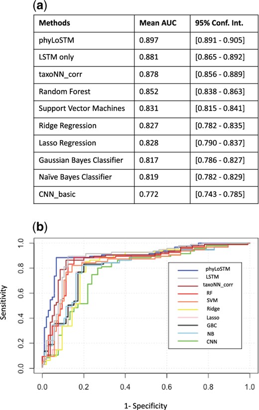
Performance on the test sets of the simulated study. (a) Table illustrating mean AUC and 95% confidence intervals of the prediction models. (b) ROC curve showing the performance of the prediction models on the simulated study

However, we also compared with machine learning models employed at single time point (in our case the first time point) which gave us results as follows: the stratified CNN, taxoNN_corr approach gave an AUC of 0.878. The other machine learning methods like RF and SVM with AUCs 0.852 and 0.831 respectively, performed relatively better than GBC and NB (AUC = 0.817, 0.819 respectively) due to their tree-based structure, rendering their ability to capture non-linearity in the data. Ridge regression and Lasso regression performed comparable to each other with AUC of 0.827. The most under-performing method was a basic CNN framework, with an AUC of 0.772 as it overlooked spatial similarity in the OTU data. It was observed that, there was a clear out-performance of phyLoSTM with a percentage increase in AUC ranging from about 5% as compared to Random Forest to about 16% for the least efficient performing method CNN_basic. The computation time taken by our method on an NVIDIA Tesla P100 GPU with 16 GB of RAM for ensemble of neural networks for feature extraction was 9.35 s. The initial ordering of the input OTU data took 1.27 s. The LSTM network took 400 epochs to learn, where each iteration took 12.29 s.

3.2.2 Real studies

DIABIMMUNE three country cohort

In this section, we present results on the training and test sets of the three country DIABIMMUNE cohort. We filtered the data in the study, eliminating OTUs that had a zero proportion in all individuals and thereby obtained 534 OTUs for the study after this filtering. Illustration of how the heatmaps are sorted and rearranged based on the correlations between the OTUs in each cluster are provided in Supplementary Figures S1–S3. We selected three food allergy types as the study outcomes, that were Peanut Allergy with 33 cases, Egg Allergy with 148 cases and Milk allergy with 188 cases. We also combined these outcomes together to constitute an overall allergy outcome with 251 cases.

Results for cross-validation on training set: The results for the dataset taking 10-fold cross validation on the training set of the three country DIABIMMUNE cohort taking only OTU data of the cohort, are presented in Figure 4. We plotted the 95% confidence intervals (CI) for each of the methods for the three individual outcomes (Fig. 4b–d), as well as the overall allergy outcome (Fig. 4a). The mean AUC values obtained for our proposed phyLoSTM method were 0.665 (95% CI: 0.659-0.670) for the egg allergy outcome, 0.559 (95% CI: 0.552-0.564) for the peanut allergy outcome and 0.735 (95% CI: 0.728-0.743) for the milk allergy outcome. However, for the overall outcome the mean AUC showed an increment to 0.745 (95% CI: 0.741-0.748). Our proposed model was followed in performance by LSTM approach.

Fig. 4.

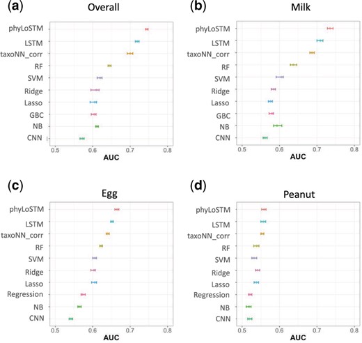
95% confidence intervals obtained for the mean AUC values for 10 times 10-fold cross validation on the training set for the DIABIMMUNE three country cohort, (a) overall allergy outcome, (b) milk allergy outcome, (c) egg allergy outcome and (d) peanut allergy outcome

Results for test set: We calculated the results on the test set of the study (tabulated in Table 1). We tabulated the results separately on each of the allergy outcomes and the overall allergy outcome. In each of these outcomes, we divided performance in two categories: The first category was model performance on test set containing only the OTU data and the second category was test set containing OTU data along with the environmental variables. We observed that the phyLoSTM outperformed all the other approaches in terms of the AUC values with AUC 0.712 for overall allergy, 0.698 for milk allergy, 0.647 for egg allergy and 0.552 for peanut allergy. Also, due to the significant association of some of the environmental variables with the outcome, we saw a spike in performance upon adding the environmental variables to the OTU data in the input with performance as high as 0.762 for overall allergy, 0.741 for milk allergy, 0.673 for egg allergy and 0.585 for peanut allergy.

Table 1.

AUC values tabulated for various machine learning methods on test set of DIABIMMUNE three country dataset (Columns 2-9) and DiGiulio study (Columns 10-11)

Methods	Overall allergy		Milk allergy		Egg allergy		Peanut allergy		Preterm birth
	AUC w/o env variables	AUC with env variables	AUC w/o env variables	AUC with env variables	AUC w/o env variables	AUC with env variables	AUC w/o env variables	AUC with env variables	AUC w/o env variables	AUC with env variables
phyLoSTM	0.712	0.762	0.698	0.741	0.647	0.673	0.552	0.585	0.695	0.713
LSTM	0.709	0.734	0.672	0.715	0.632	0.653	0.553	0.569	0.687	0.692
taxoNNcorr	0.688	0.711	0.655	0.691	0.627	0.641	0.550	0.561	0.662	0.678
RF	0.625	0.639	0.619	0.637	0.601	0.619	0.548	0.552	0.658	0.659
SVM	0.600	0.611	0.589	0.605	0.574	0.601	0.531	0.532	0.644	0.641
Ridge	0.601	0.607	0.575	0.584	0.571	0.598	0.539	0.541	0.633	0.634
Lasso	0.596	0.603	0.562	0.576	0.572	0.600	0.533	0.538	0.632	0.630
GBC	0.589	0.601	0.571	0.580	0.553	0.569	0.517	0.521	0.629	0.631
NB	0.600	0.609	0.585	0.593	0.545	0.558	0.501	0.518	0.623	0.624
CNN_basic	0.560	0.569	0.553	0.561	0.527	0.537	0.513	0.520	0.601	0.604

Note: For DIABIMMUNE three country dataset, the results are reported on overall allergy and individual allergies considering model performance without (w/o) including environmental variables and with including environmental variables. For DiGiulio study, the results are reported on preterm delivery output considering model performance without (w/o) including environmental variables and with including environmental variables. Note that the first row in bold shows the improvement in the performance of the proposed phyLoSTM for both studies.

DiGiulio case–control study

To validate phyLoSTM’s robustness on another independent dataset, we obtained results on the test set, as well as, did a cross-validation on training test of the DiGiulio study. The results for the dataset with 10 times 10-fold cross validation on the training set of this dataset considering OTUs as input are presented in Supplementary Figure S6. For the results on the test set, as shown in the last two columns of Table 1, we observed a consistent improvement in performance through our phyLoSTM model on the DiGiulio study, followed in performance by Random Forest approach amongst the conventional machine learning algorithms. On the test set of this study taking OTUs and environmental variables together as the input and preterm delivery as the output, we obtained an AUC of 0.713 with the phyLoSTM modeling, followed by LSTM with an AUC of 0.692. Random Forest methodology performed the best amongst the conventional machine learning models with an AUC of 0.659, which was about 8% less than the phyLosTM modeling, followed by SVM with an AUC of 0.641, Ridge and Lasso regression with AUCs of 0.634 and 0.630 respectively, followed by GBC and NB with AUCs of 0.631 and 0.624. A basic CNN modeling performed poorly with the lowest AUC of 0.604.

4 Discussion

We have proposed a novel modeling named ‘phyLoSTM’ on longitudinal microbiome sequencing data. As discussed in Section 1, longitudinal microbiome sequencing analysis for disease risk prediction is clinically more relevant as it incorporates change in microbiome data temporally, due to infections/diet/environmental factors of the subject. Such a comprehensive temporal analysis provides insight on both single timepoint factors affecting disease risk, as well as, data trend over time affecting microbiome composition and prediction efficiency. Extensive analysis on simulation studies, as well as, on two human microbiome studies with different allergy and preterm delivery outcomes have shown that the proposed model is efficient while predicting disease status in longitudinal studies. The results from both simulation and real studies showed that the taxonomic structure-based stratification with spatial correlation of the OTU data helps in efficient extraction of feature sets from the microbiome data at each time point and phyLoSTM further enhances the performance taking in consideration the temporal dependencies of the microbiome profiles. In Supplementary Figure S4 and Supplementary Tables S10 and S11, the performance spike in AUC using phyLoSTM for capturing temporal dependency as compared to using taxoNN_corr as well as other conventional machine learning models at individual time points shows the competence of our approach. Also, upon experimenting with only LSTM networks, where input OTUs are given unstructured to the modeling, the temporal aspect was captured well, however, there was a significant loss in performance as can be seen in Table 1, which validates our usage of CNN model for feature extraction before providing the feature set to an LSTM network. Other methods such as, Random Forests which have proven to work well with non-linear data (Ryo and Rillig, 2017), performed slightly better than Naive Bayes and Gaussian Bayes Classifier methods while predicting the risk of disease.

In the proposed modeling, we also dealt with imbalance in the microbiome data at each time point. Since the cases in our microbiome data were lower in number than the controls, hence, we enhanced the weight associated with the class having less number of samples (cases) and thereby ensured imbalance in the dataset is mitigated which helped in improving AUC values. Significant improvement was noted for peanut allergy where the imbalance between cases and controls was in the ratio 1:20. A comparative analysis of AUC values before and after tackling imbalance using weight balancing is shown in Supplementary Table S5. Our methodology is also consistent in performance across both 16s and metagenomic datasets as shown in Supplementary Table S8, validating the robustness of our approach to difference in OTU generation pipeline.

We also analyzed the methods in the literature that propose machine learning techniques for longitudinal microbiome dataset (Metwally et al., 2019) using an autoencoder network for feature extraction and applying an LSTM for predicting overall allergy in the DIABIMMUNE dataset. We differ in their approach of feature extraction and also we provide an enhanced performance with AUCs of 0.762 as opposed to the AUC of 0.67 obtained in (Metwally et al., 2019). We also do an exhaustive evaluation on each of the individual allergy tests to show the robustness of our approach on various outcomes and varying case-control distributions. Upon comparing taxoNN_corr approach with other feature extraction techniques (refer Supplementary Table S7), we also observed higher AUC validating the effectiveness of a stratified CNN approach for feature extraction.

There are certain limitations for our study. In the simulated study design, we take the liberty of using 32 OTUS and 3 interaction terms to approximate OTU association and interactions in a real dataset. However, an exhaustive analysis to conclude the number of associated OTUs needs to be performed to approximate real data well. The simulated study design also employs time as a linear covariate. The third limitation is, the requirement of having sufficient samples for the feature extraction at each time point limits our real study division into six and four timepoints respectively. In the future, we plan to explore more studies containing large number of samples at each time point to analyze temporal effects in the data without losing information due to grouping. Our current approach was also limited to a fixed outcome definition such as, case versus control, response versus no response. For our analysis, we consider phylum level stratification in taxoNN in both studies, due to presence of adequate number of OTUs in phylum level which is required for efficient model training. However, in the future studies, it will be interesting to observe datasets which have adequate OTUs in other taxonomy levels such as class and order along with phylum level (Supplementary Table S9). In the future, it would also be interesting to analyze our approach on datasets with varying outcomes for the same subject at different timepoints. Analyzing non-linear relationship along time can also be a good area for future scope.

In conclusion, the strength of our methodology lies in efficient feature extraction from longitudinal microbiome data through a two-step CNN-LSTM modeling called phyLoSTM. Exhaustive temporal analysis helped in improving the prediction accuracy in both simulated and real studies. Our methodology can be extended to various longitudinal studies, where data exhibits spatial correlations at individual time points and changes in data pattern contribute to outcome prediction.

Funding

Wei Xu was funded by Natural Sciences and Engineering Research Council of Canada (NSERC Grant RGPIN-2017-06672), Crohn’s and Colitis Canada (CCC Grant CCC-GEMIII), and Helmsley Charitable Trust. Divya Sharma was supported by NSERC Grant RGPIN-2017-06672 and CCC Grant CCC-GEMIII.

Conflict of Interest: none declared.