Transformation and differential abundance analysis of microbiome data incorporating phylogeny

Abstract

Motivation

Microbiome data have proven extremely useful for understanding microbial communities and their impacts in health and disease. Although microbiome analysis methods and standards are evolving rapidly, obtaining meaningful and interpretable results from microbiome studies still requires careful statistical treatment. In particular, many existing and emerging methods for differential abundance (DA) analysis fail to account for the fact that microbiome data are high-dimensional and sparse, compositional, negatively and positively correlated and phylogenetically structured. To better describe microbiome data and improve the power of DA testing, there is still a great need for the continued development of appropriate statistical methodology.

Results

In this article, we propose a model-based approach for microbiome data transformation, and a phylogenetically informed procedure for DA testing based on the transformed data. First, we extend the Dirichlet-tree multinomial (DTM) to zero-inflated DTM for multivariate modeling of microbial counts, addressing data sparsity and correlation and phylogeny among bacterial taxa. Then, within this framework and using a Bayesian formulation, we introduce posterior mean transformation to convert raw counts into non-zero relative abundances that sum to one, accounting for the compositionality nature of microbiome data. Second, using the transformed data, we propose adaptive analysis of composition of microbiomes (adaANCOM) for DA testing by constructing log-ratios adaptively on the tree for each taxon, greatly reducing the computational complexity of ANCOM in high dimensions. Finally, we present extensive simulation studies, an analysis of HMP data across 18 body sites and 2 visits, and an application to a gut microbiome and malnutrition study, to investigate the performance of posterior mean transformation and adaANCOM. Comparisons with ANCOM and other DA testing procedures show that adaANCOM controls the false discovery rate well, allows for easy interpretation of the results, and is computationally efficient for high-dimensional problems.

Availability and implementation

The developed R package is available at https://github.com/ZRChao/adaANCOM. For replicability purposes, scripts for our simulations and data analysis are available at https://github.com/ZRChao/Papers_supplementary.

Supplementary information

Supplementary data are available at Bioinformatics online.

1 Introduction

To better understand the role of microbiome for human health, large-scale collaborative projects, including MetaHIT (Ehrlich et al., 2011) and the Human Microbiome Project (Huttenhower et al., 2012), have been carried out worldwide over the past 15 years. Analyses of the large amounts of data generated from these projects and other studies pose major computational and statistical challenges, and have spurred the development of numerous bioinformatic tools (Bolyen et al., 2019). For example, following 16s rRNA sequencing and quality checking, sequence reads are usually clustered into Operational Taxonomic Units (OTUs), based on sequence similarity. OTU picking is then followed by assigning representative OTU sequences into taxonomic levels. In addition to an OTU table and/or a taxonomy table, bioinformatic processing of micriobiome data often provides a phylogenetic tree that reflects the evolutionary relationships among bacterial taxa. After data preprocessing, different statistical analyses can be conducted for different purposes (Knight et al., 2018). This article concerns model-based transformation of microbiome abundance data and differential abundance (DA) testing based on the transformed data.

Although microbiome data have proven extremely useful, obtaining meaningful and interpretable results from microbiome studies requires careful statistical treatment. In particular, intrinsic characteristics of microbiome data can cause misleading results if not addressed (Weiss et al., 2017). First, the microbiome represents hundreds or even thousands of microbes, some of which are dominant but most are rare, and hence microbiome abundance data (that is, multivariate taxon counts) are high-dimensional, over-dispersed and sparse with a large proportion of zeros. Second, the possible interactions between microbes can be both competitive and synergistic, and there is a phylogenetic tree relating all bacterial taxa. As a consequence, microbiome taxon counts are both negatively and positively corrected, and are phylogenetically structured. Third, due to technical reasons, microbiome data are compositional containing only relative information. It is thus challenging to draw inferences on the total abundance in the ecosystem based on specimen-level taxon abundance data. This is known as the compositional bias (Kumar et al., 2018; Lin and Peddada, 2020).

To address the deficiencies of traditional statistical methods, a variety of methods have been proposed. In particular, popular models for describing multivariate taxon counts include the Dirichlet-multinomial (DM) (La Rosa et al., 2012), the generalized DM (GDM) (Zhang et al., 2017) and the zero-inflated GDM (ZIGDM) (Tang and Chen, 2019), with increasing level of flexibility. To better describe microbiome data, Wang and Zhao (2017) proposed an extension of DM, called the Dirichlet-tree multinomial (DTM), by incorporating the phylogenetic tree information. It is worth noting that GDM is a special case of DTM when the tree is completely skewed binary. There are many other methods for phylogeny-aware analyses of microbiome data (Washburne et al., 2018). For example, UniFrac uses the phylogeny to construct distances between microbial communities (Lozupone et al., 2011). Furthermore, procedures for distance-based hypothesis testing, such as MiRKAT (Zhao et al., 2015) and OMiAT (Koh et al., 2017), modulate relative contributions from microbial abundance and phylogenetic information. The above phylogenetically informed methods either assess the overall patterns in microbiome variation or explain the variation of a phenotype, but, at individual taxon level, amending DA testing using a phylogeny is less developed in the literature (Liu et al., 2020).

Identifying bacterial taxa that are differentially abundant between conditions of interest is challenging because of the compositional nature of microbiome data. To correct for the compositional bias, many of the methods for DA testing involve a scaling normalization step by multiplying microbial counts by some scale factors, such as trimmed mean of M-values (TMM) in edgeR (Robinson et al., 2010), median of ratios in DESeq2 (Love et al., 2014) and cumulative-sum scaling (CSS) in metagenomeSeq (Paulson et al., 2013). However, they all implicitly assume that most taxa are not differentially abundant. Furthermore, when the count matrix has a high fraction of zeros, scaling can overestimate or underestimate the community diversity, distort the correlations among taxa and even fail to provide a solution (Kumar et al., 2018; Weiss et al., 2017).

An attractive alternative to scaling is log-ratio transformation which is a starting point in traditional analysis of compositional data. Often, the additive log-ratios, centered log-ratios and isometric log-ratios are used (Egozcue et al., 2003). After a log-ratio transformation is applied, standard statistical tests, such as the two sample t-test and Wilcoxon rank-sum test, can effectively detect for differences between microbial communities in a compositionally aware manner. Analysis of composition of microbiomes (ANCOM), which was proposed specifically for microbiome datasets, is a recommended method for DA testing (Mandal et al., 2015). It carries out tests by comparing the log-ratios of the abundance of each taxon to the abundance of all the other taxa. As discussed in the next section, however, ANCOM is computationally intensive and tends to have a high false discovery rate. In this article, we propose a means for improving ANCOM by incorporating the phylogenetic tree information.

Like scaling, zero counts pose a challenge for methods that depend on log-ratio transformation, because we cannot take the log of zeros. One way to address this issue is to transform raw counts into non-zero relative abundances using a Bayesian treatment. For example, assuming a multinomial for counts and a Dirichlet prior for the underlying proportions, the posterior means for the proportions always sum to one and lie between the prior mean and the maximum likelihood estimate corresponding to the relative frequencies (Martín-Fernández et al., 2015; Liu et al., 2020). Posterior mean transformation includes as a special case the pseudo count method, which adds a small value (for example, 0.5) to all counts. In this case, a uniform prior is implicitly used. In this article, we propose a flexible Bayesian formulation to perform posterior mean and then log-ratio transformation, taking account of high-dimensionality, compositionality, data sparsity and correlation and phylogeny among taxa.

In this article, we first extend DTM to zero-inflated DTM (ZIDTM). We develop an efficient expectation-maximization algorithm for maximum likelihood estimation. Within this framework, we derive the posterior mean transformation at different levels of granularity. Then, based on the transformed data, we propose adaptive ANCOM (adaANCOM) by constructing log-ratios adaptively according to the tree for each taxon. Comparison with ANCOM shows that adaANCOM scales better for high dimensions, allows for easier interpretation of the results, and controls the false discovery rate potentially better. Finally, we investigate the performance of adaANCOM using extensive simulation studies and two real data applications.

2 Materials and methods

2.1 Zero-inflated Dirichlet-tree-multinomial (ZIDTM) distribution

The most often used multivariate distribution for over-dispersed OTU counts is the Dirichlet-multinomial (DM), which is a compound multinomial with probabilities from a Dirichlet prior (La Rosa et al., 2012). Suppose $\mathit{y}={(y_1,\dots ,y_K)}^T$ is the count vector for a sample with K OTUs. The probability mass function of the multinomial is given as

$$f_M(\mathit{y};\mathit{p})=\frac{\Gamma (y^{+}+1)}{\prod _{k=1}^K\Gamma (y_k+1)}\prod _{k=1}^K{p}_k^{y_k},$$

where $y^{+}=\sum _{k=1}^K{y}_k,\hspace{0.17em}\Gamma (·)$ is the gamma function, and $\mathit{p}={(p_1,\dots ,p_K)}^T$ is the vector of OTU probabilities with $p_k>0$ and $\sum _{k=1}^K{p}_k=1$⁠. The Dirichlet distribution for the underlying composition is indexed by a vector of positive parameters, $\mathit{\alpha }={({\alpha }_1,\dots ,{\alpha }_K)}^T,{\alpha }_k>0$⁠, and has density function

$$f_D(\mathit{p};\mathit{\alpha })=\frac{\Gamma ({\alpha }^{+})}{\prod _{k=1}^K\Gamma ({\alpha }_k)}\prod _{k=1}^K{p}_k^{{\alpha }_k},$$

where ${\alpha }^{+}=\sum _{k=1}^K{\alpha }_k$⁠. The Dirichlet-multinomial then takes the form

$$\begin{array}{c}{f}_{DM}(\mathit{y};\mathit{\alpha })=\int f_M(\mathit{y};\mathit{p})f_D(\mathit{p};\mathit{\alpha })d\mathit{p}\\ =\frac{\Gamma (y^{+}+1)\Gamma ({\alpha }^{+})}{\Gamma (y^{+}+{\alpha }^{+})}\prod _{k=1}^K\frac{\Gamma (y_k+{\alpha }_k)}{\Gamma (y_k+1)\Gamma ({\alpha }_k)}.\end{array}$$

One can reparametrize DM as $\theta =1/(1+{\alpha }^{+})$ and ${({\alpha }_1/{\alpha }^{+},\dots ,{\alpha }_K/{\alpha }^{+})}^T$⁠. Hence, DM is multinomial augmented with one additional parameter θ. We call θ the over-dispersion parameter.

We first extend DM to zero-inflated DM (ZIDM). There is an important relation between the Dirichlet, the gamma and the beta distribution. Suppose that $Z_1,\dots ,Z_K$ are independent gamma variables with the same scale parameter, $Z_k\sim \mathit{Gamma}({\alpha }_k,\lambda )$⁠, with density function

$$f_G(z_k;{\alpha }_k,\lambda )=\frac{1}{\Gamma ({\alpha }_k){\lambda }^{{\alpha }_k}}{z}_k^{{\alpha }_k-1}{e}^{-z_k/\lambda }.$$

Let $X_k=Z_k/\sum _{j=1}^K{Z}_j,W_k=Z_k/\sum _{j=k}^K{Z}_j$⁠, for $k=1,\dots ,K-1$⁠, and let $X_K=1-\sum _{j=1}^{K-1}{X}_j$⁠. Then the joint distribution of $\mathit{X}={(X_1,\dots ,X_K)}^T$ is the Dirichlet distribution with parameter vector $\mathit{\alpha }$⁠, and W_k are independent beta variables, $W_k\sim \mathit{Beta}({\alpha }_k,{\alpha }_k^{+})$⁠, with density function

$$f_B(w_k;{\alpha }_k,{\alpha }_k^{+})=\frac{1}{\mathcal{B}({\alpha }_k,{\alpha }_k^{+})}{w}_k^{{\alpha }_k-1}{(1-w_k)}^{{\alpha }_k^{+}-1},$$

where ${\alpha }_k^{+}=\sum _{j=k+1}^K{\alpha }_j$⁠, and $\mathcal{B}(·,·)$ is the beta function. Furthermore, X₁ = W₁, and $X_k=W_k\prod _{j=1}^{k-1}(1-W_j)$⁠, for $k=2,\dots ,K-1$⁠. Denote by $h(·)$ the transformation from $\mathit{W}$ to $\mathit{X}$⁠. Then, we can rewrite

$$f_{DM}(\mathit{y};\mathit{\alpha })=\int f_M(\mathit{y};h(\mathit{w}))\prod _{k=1}^{K-1}{f}_B(w_k;{\alpha }_k,{\alpha }_k^{+})d\mathit{w}.$$

By introducing zero-inflation to W_k, we define ZIDM as

$$f_{\mathit{ZIDM}}(\mathit{y};\mathit{\pi },\mathit{\alpha })=\int f_M(\mathit{y};h(\mathit{w}))\prod _{k=1}^{K-1}{f}_{\mathit{ZIB}}(w_k;{\pi }_k,{\alpha }_k,{\alpha }_k^{+})d\mathit{w},$$

where

$$f_{\mathit{ZIB}}(w_k;{\pi }_k,{\alpha }_k,{\alpha }_k^{+})={\pi }_k\delta (0)+(1-{\pi }_k)f_B(w_k;{\alpha }_k,{\alpha }_k^{+}).$$

Here, π_k is the probability of zero-inflation in the kth component, and $\delta (·)$ is the Dirac delta function. Replacing $\mathit{Beta}({\alpha }_k,{\alpha }_k^{+})$ by $\mathit{Beta}({\alpha }_k,{\beta }_k)$ leads to the zero-inflated generalized DM (ZIGDM, Tang and Chen (2019)), where ${\beta }_k>0$ are additional free parameters. Note that, in contrast to DM, GDM and ZIDM are not exchangeable, in the sense that they depend on the ordering of the OTUs. We call this the ‘matching problem’.

Now we extend DTM (Wang and Zhao (2017)) to ZIDTM. Suppose the relationship among OTUs is encoded in a tree, $\mathcal{T}$⁠, composing of an internal node set $\mathcal{V}$ and a leaf node set $\mathcal{L}$⁠. For each $v\in \mathcal{V}$⁠, let ${\mathcal{C}}_v$ be the set of child nodes of v, ${\mathit{y}}_v$ the vector of counts corresponding to ${\mathcal{C}}_v$ and $y_v^{+}=\sum _{u\in {\mathcal{C}}_v}{y}_u$⁠. By assuming that ${\mathit{y}}_v$ conditional on $y_v^{+}$ are independent across the internal nodes, the DTM distribution is defined as the product of DM distributions that factorize over the tree

$$f_{\mathit{DTM}}(\mathit{y};{\mathit{\alpha }}_v,v\in \mathcal{V})=\prod _{v\in \mathcal{V}}{f}_{DM}({\mathit{y}}_v;y_v^{+},{\mathit{\alpha }}_v),$$

where ${\mathit{\alpha }}_v$ are vectors of positive scalars. It is easy to see that GDM is a special case of DTM, when the tree structure is restricted to a binary cascade. Note that incorporating the phylogeny posits an ordering of OTUs, and thus removes the matching problem for GDM. Replacing DMs by ZIDMs then defines the ZIDTM:

$$f_{\mathit{ZIDTM}}(\mathit{y};{\mathit{\pi }}_v,{\mathit{\alpha }}_v,v\in \mathcal{V})=\prod _{v\in \mathcal{V}}{f}_{\mathit{ZIDM}}({\mathit{y}}_v;y_v^{+},{\mathit{\pi }}_v,{\mathit{\alpha }}_v)$$

where ${\mathit{\pi }}_v$ are vectors with length $\left|{\mathcal{C}}_v\right|-1$ for probabilities of zero-inflation. Conceptually, ZIDTM inherits the matching problem from ZIDM. However, computationally, the problem is alleviated when the cardinality of ${\mathcal{C}}_v,\hspace{0.17em}\left|{\mathcal{C}}_v\right|$⁠, is small for each $v\in \mathcal{V}$⁠. As we will see, this is the case for binary trees.

Figure 1 illustrates the idea. As mentioned above, a distinctive property of DTM (and hence ZIDTM) is that the correlations between counts on tree nodes can be simultaneously negative and positive; see Supplementary Figure S1.

Fig. 1.

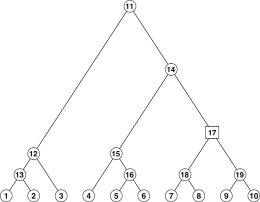
A binary tree with K = 10 leaves. Here $\mathcal{L}=\{1,2,\dots ,10\},\hspace{0.17em}\mathcal{V}=\{11,12,\dots ,19\}$⁠. For illustration, ${\mathcal{C}}_{17}=\{18,19\},{\mathit{y}}_{17}={(y_{18},y_{19})}^T$ and $y_{17}^{+}=y_{18}+y_{19}$⁠. Given $y_{17}^{+},\hspace{0.17em}{\mathit{y}}_{17}$ has a DM or ZIDM distribution. The factorization over internal nodes means that these conditional distributions are independent

2.1.1 Maximum likelihood estimation for ZIDTM

We estimate the unknown parameters of ZIDTM by maximum likelihood, using the expectation-maximization (EM) algorithm. Let $\mathit{\theta }=\{{\mathit{\alpha }}_v,{\mathit{\pi }}_v,v\in \mathcal{V}\}$⁠. Assume that ${\mathcal{C}}_v=\{1,\dots ,K_v\}$⁠, where $K_v=\left|{\mathcal{C}}_v\right|$⁠. With n observations, ${\mathit{y}}^1,\dots ,{\mathit{y}}^n$⁠, the complete data log-likelihood function, ignoring the constant terms, is given by

$$l(\mathit{\theta })=\sum _{i=1}^n\sum _{v\in \mathcal{V}}\sum _{k=1}^{K_v-1}\left\{l_1({\delta }_{vk}^i,{\pi }_{vk})+l_2({\delta }_{vk}^i,w_{vk}^i,{\alpha }_{vk},{\alpha }_{vk}^{+})\right\},$$

where ${\delta }_{vk}^i$ is the indicator of zero-inflation,

$$l_1({\delta }_{vk}^i,{\pi }_{vk})={\delta }_{vk}^i\hspace{0.17em}\text{log}\hspace{0.17em}{\pi }_{vk}+(1-{\delta }_{vk}^i)\hspace{0.17em}\text{log}(1-{\pi }_{vk}),$$

and

$$\begin{array}{c}{l}_2({\delta }_{vk}^i,w_{vk}^i,{\alpha }_{vk},{\alpha }_{vk}^{+})=(1-{\delta }_{vk}^i)\{-\text{log}\hspace{0.17em}\mathcal{B}({\alpha }_{vk},{\alpha }_{vk}^{+})+\hfill \\ ({\alpha }_{vk}-1)\hspace{0.17em}\text{log}\hspace{0.17em}{w}_{vk}^i+({\alpha }_{vk}^{+}-1)\hspace{0.17em}\text{log}(1-w_{vk}^i)\}.\hfill \end{array}$$

In the E-step, we compute the expectation of $l(\mathit{\theta })$ with respect to the posterior distribution of $({\delta }_{vk}^i,w_{vk}^i)|{\mathit{y}}_v^i$⁠, which is indexed by the current value of $\mathit{\theta }$⁠, and get the Q-function

$$Q(\mathit{\theta })=\sum _{i=1}^n\sum _{v\in \mathcal{V}}\sum _{k=1}^{K_v-1}E\{l_1({\delta }_{vk}^i,{\pi }_{vk})+l_2({\delta }_{vk}^i,w_{vk}^i,{\alpha }_{vk},{\alpha }_{vk}^{+})\}.$$

Define ${\delta }_{vk}^{i*}=E({\delta }_{vk}^i|{\mathit{y}}_v^i),\hspace{0.17em}{R}_{vk}^{i*}=E(\text{log}\hspace{0.17em}{w}_{vk}^i|{\mathit{y}}_v^i,{\delta }_{vk}^i=0)$ and $S_{vk}^{i*}=E\{\hspace{0.17em}\text{log}(1-w_{vk}^i)|{\mathit{y}}_v^i,{\delta }_{vk}^i=0\}$⁠. We have

$$\begin{array}{c}\begin{array}{c}{\delta }_{vk}^{i*}=\{\begin{array}{cc}0,\hfill & y_{vk}^i>0,\hfill \\ \frac{{\pi }_{vk}}{{\pi }_{vk}+(1-{\pi }_{vk})\frac{\mathcal{B}({\alpha }_{vk}^{i*},{\alpha }_{vk}^{i*+})}{\mathcal{B}({\alpha }_{vk},{\alpha }_{vk}^{+})}},\hfill & y_{vk}^i=0,\hfill \end{array}\hfill \end{array}\\ R_{vk}^{i*}=\psi ({\alpha }_{vk}^{i*})-\psi ({\alpha }_{vk}^{i*+}),\end{array}$$

and

$$\begin{array}{c}{S}_{vk}^{i*}=\psi ({\alpha }_{vk}^{i*+})-\psi ({\alpha }_{vk}^{i*}+{\alpha }_{vk}^{i*+}),\hfill \end{array}$$

where ${\alpha }_{vk}^{i*}={\alpha }_{vk}+y_{vk}^i,\hspace{0.17em}{\alpha }_{vk}^{i*+}=\sum _{j=k+1}^{K_v}{\alpha }_{vk}^{i*}$ and $\psi (·)$ is the digamma function. Hence,

$$Q(\mathit{\theta })=\sum _{i=1}^n\sum _{v\in \mathcal{V}}\sum _{k=1}^{K_v-1}\{Q_1({\pi }_{vk},{\delta }_{vk}^i)+Q_2({\alpha }_{vk},{\alpha }_{vk}^{+},R_{vk}^{i*},S_{vk}^{i*})\},$$

where

$$Q_1({\pi }_{vk},{\delta }_{vk}^i)={\delta }_{vk}^{i*}\hspace{0.17em}\text{log}({\pi }_{vk})+(1-{\delta }_{vk}^{i*})\hspace{0.17em}\text{log}(1-{\pi }_{vk}),$$

and

$$\begin{array}{c}{Q}_2({\alpha }_{vk},{\alpha }_{vk}^{+},R_{vk}^{i*},S_{vk}^{i*})=(1-{\delta }_{vk}^{i*})\{-\text{log}\hspace{0.17em}\mathcal{B}({\alpha }_{vk},{\alpha }_{vk}^{+})+\hfill \\ ({\alpha }_{vk}-1)R_{vk}^{i*}+({\alpha }_{vk}^{+}-1)S_{vk}^{i*}\}.\hfill \end{array}\hspace{0.17em}$$

In the M-step, we maximize $Q(\mathit{\theta })$ with respect to $\mathit{\theta }$⁠. Clearly, parameters in Q₁ and Q₂ can be optimized separately, and each can be carried out in parallel. To address the matching problem, at each internal node, we fit a separate ZIDM model for each possible ordering of the $\left|{\mathcal{C}}_v\right|$ taxa, and select the best fitted model. Compared with GDM or ZIDM, the computational cost for ZIDTM reduces from $O(|\mathcal{L}|!)$ to $O(\sum _{v\in \mathcal{V}}|{\mathcal{C}}_v|!)$⁠.

In the rest of this article, we restrict our attention to binary trees, in which $\left|{\mathcal{C}}_v\right|=2$ for all $v\in \mathcal{V}$⁠. In this case, the Dirichlet, the multinomial, the DM and the ZIDM reduce to the beta, the binomial (BN), the beta-binomial (BB) and the zero-inflated beta-binomial (ZIBB), respectively. Then ZIDTM is a product of ZIBBs, and its computational burden grows linearly in $\left|\mathcal{L}\right|$⁠, which is the fastest possible.

Note that, for an internal node, if the count for one of its children is always non-zero, which often happens for a common taxon, then the probability of zero-inflation for that child is zero. In the extreme case, the ZIDM for an internal node reduces to a DM when the counts for its children are all non-zero. In practice, the observed counts for a child node are likely to be zero (that is, the corresponding taxon be absent) in some samples, then our estimation procedure provides an estimated probability of zero-inflation for this node. In other words, the fitting algorithm for ZIDTM decides the level of zero inflation adaptively from the data.

2.1.2 Posterior mean transformation

The Dirichlet prior is popular mainly because it is conjugate to the multinomial distribution. This allows us to estimate the underlying proportions from a Bayesian perspective. In the case of DM, the posterior mean has the form

$$E_{DM}(p_k|\mathit{y})=\frac{{\alpha }_k+y_k}{\sum _{j=1}^K(y_j+{\alpha }_j)}.$$

We can estimate the unknown parameters by maximizing the evidence, that is, the data likelihood. The estimated parameters are then converted into ‘pseudo data’ which can then be ‘merged’ with the observed data. This method has the advantage of producing non-zero proportions for zero counts. A related but ad hoc procedure is to add a pseudo count (such as 0.5) to the raw counts, and use the sample proportions.

The situation is much more complex in the presence of zero-inflation. However, when the count vector has just two components (K = 2), there is an explicit closed-form solution. It is easy to verify that

$$E_{BB}(p_1|\mathit{y})=\frac{{\alpha }_1+y_1}{{\alpha }_1+{\alpha }_2+y_1+y_2},$$

and

$$E_{\mathit{ZIBB}}(p_1|\mathit{y})=\frac{(1-B_0)B_1}{B_0\mathcal{B}({\alpha }_1,{\alpha }_2)+(1-B_0)B_2},$$

where $B_0=\pi I(y_1=0),\hspace{0.17em}{B}_1=\mathcal{B}(1+{\alpha }_1+y_1,{\alpha }_2+y_2)$ and $B_2=\mathcal{B}({\alpha }_1+y_1,{\alpha }_2+y_2)$⁠.

For binary trees, these are naturally extended to DTM and ZIDTM. At each internal node $v\in \mathcal{V}$⁠, we have

$$E_{BB}(p_{v1}|{\mathit{y}}_v)=\frac{{\alpha }_{v1}+y_{v1}}{{\alpha }_{v1}+{\alpha }_{v2}+y_{v1}+y_{v2}},$$

(1)

and

$$E_{\mathit{ZIBB}}(p_{v1}|{\mathit{y}}_{\mathit{v}})=\frac{(1-B_{v0})B_{v1}}{B_{v0}\mathcal{B}({\alpha }_{v1},{\alpha }_{v2})+(1-B_{v0})B_{v2}},$$

(2)

where $B_{v0},B_{v1}$ and $B_{v2}$ are similarly defined.

Correctly specifying the model at each internal node can have a large effect on the quality of the posterior estimates. We propose a two-stage likelihood-ratio test. First, we assume that count data at $v\in \mathcal{V}$ are not zero-inflated, fit a BB model and test for over-dispersion. For nodes without over-dispersion, counts are transformed into sample proportions after adding a common constant of 0.5, that is, using (1) with ${\alpha }_{v1}={\alpha }_{v2}=0.5$⁠. Second, nodes with over-dispersion are refitted by a ZIBB model, and are tested for zero-inflation. Counts are then transformed by (2) in the presence of zero-inflation, and (1) otherwise. Denote by ${\widehat{\mathit{p}}}_v={({\widehat{p}}_{v1},1-{\widehat{p}}_{v1})}^T$ the chosen posterior estimate.

So far we have concentrated on individual internal nodes, but the results can be extended to the path level. For each node $u\in \mathcal{L}\cup \mathcal{V}$⁠, let ${\mathcal{A}}_u$ denote the ancestor node set of u, consisting all internal nodes in the path from the root node to u, and ${\mathcal{L}}_u$ the set of leaves in the same path. In Figure 1, for example, ${\mathcal{A}}_1={\mathcal{A}}_2=\{11,12,13\},\hspace{0.17em}{\mathcal{A}}_3=\{11,12\},\hspace{0.17em}{\mathcal{L}}_{11}=\mathcal{L},\hspace{0.17em}{\mathcal{L}}_{12}=\{1,2,3\},\hspace{0.17em}{\mathcal{L}}_{13}=\{1,2\}$⁠. We define

$$q_u=\prod _{v\in {\mathcal{A}}_u}{\widehat{p}}_v.$$

(3)

Suppose that $\mathcal{U}$ is a set of nodes such that ${\cup }_{u\in \mathcal{U}}{\mathcal{L}}_u=\mathcal{L}$ and ${\mathcal{L}}_u\cap {\mathcal{L}}_{u\prime }=\varnothing$⁠, for $u\ne u\prime$⁠. Then, it is easy to see that $\sum _{u\in \mathcal{U}}{q}_u=1$⁠. In particular, we have $\sum _{l\in \mathcal{L}}{q}_l=1$⁠. This is the so-called ‘phylogeny-aware normalization’ (Liu et al., 2020).

2.2 adaANCOM

In this section, we introduce a novel method for detecting differentially abundant (DA) OTUs at the ecosystem level. Although the goal is the same as that for ANCOM, the difference being the incorporation of a phylogenetic tree whose leaf nodes correspond to these OTUs. Consider simply the two-group situation. We need to test the hypotheses

$$H_{0l}:\hspace{0.17em}\text{log}\hspace{0.17em}{\mu }_l^1=\text{log}\hspace{0.17em}{\mu }_l^2$$

for $l\in \mathcal{L}=\{1,\dots ,K\}$⁠, where ${\mu }_l^g$ is the mean absolute abundance in the ecosystem of the lth OTU from the gth group, g = 1, 2.

The main contribution of ANCOM is to use relative abundance data to perform the tests. Specifically, for each $H_{0l}$⁠, ANCOM involves testing K—1 hypotheses based on additive log-ratios, namely,

$$H_{0lm}:\hspace{0.17em}\text{log}({\mu }_l^1/{\mu }_m^1)=\text{log}({\mu }_l^2/{\mu }_m^2)$$

for all $m\ne l$⁠. To decide whether the lth OTU is differentially abundant or not, ANCOM counts the reject number among the K—1 hypotheses. It then computes the empirical distribution of these numbers, and determines a suitable cut-off. When K is large, this may result in a high false discovery rate (Weiss et al., 2017). Another drawback of ANCOM is computational: the total number of tests increases from K to $K(K-1)/2$⁠.

To speed up the computation of ANCOM while keeping its essential feature, we propose adaptive ANCOM (adaANCOM) by constructing log-ratios adaptively on the tree. The underlying assumption is that abundance difference on the log scale at an internal node passes down to its descendants. Loosely speaking, adaANCOM consists of two steps. In the first step, we test the internal node-level hypotheses

$$H_{0v}:\hspace{0.17em}\text{log}({\mu }_{v1}^1/{\mu }_{v2}^1)=\text{log}({\mu }_{v1}^2/{\mu }_{v2}^2)$$

for $v\in \mathcal{V}$⁠, where ${\mu }_{v1}^g$ and ${\mu }_{v2}^g$ are the mean absolute abundances in the ecosystem of two children of v from the gth group. For a predefined significance level α, e.g. 0.05, we obtain a set ${\mathcal{D}}_{\mathcal{V}}$ of internal nodes for which the hypotheses are rejected.

Second, for each leaf node $l\in \mathcal{L}$⁠, we calculate the log-ratio and carry out the test as follows. Define ref_l to be the sibling node of l, if ${\mathcal{A}}_l\cap {\mathcal{D}}_{\mathcal{V}}=\varnothing$⁠, and the child node of v not in ${\mathcal{A}}_l$ otherwise, where v is the node in ${\mathcal{A}}_l\cap {\mathcal{D}}_{\mathcal{V}}$ closest to the root node. Consider the null hypothesis

$$H_{0l}^{\mathit{ada}}:\hspace{0.17em}\text{log}({\mu }_l^1/{\mu }_{re{f}_l}^1)=\text{log}({\mu }_l^2/{\mu }_{re{f}_l}^2).$$

Then, adaANCOM rejects the hypothesis $H_{0l}$ if $H_{0l}^{\mathit{ada}}$ is rejected. As an illustrative example, we consider Figure 1 and assume that $D_{\mathcal{V}}=\left\{17\right\}$⁠. Then we have $re{f}_1=2,\hspace{0.17em}re{f}_2=1,\hspace{0.17em}re{f}_3=13,\hspace{0.17em}re{f}_4=16,\hspace{0.17em}re{f}_5=6,\hspace{0.17em}re{f}_6=5,\hspace{0.17em}re{f}_7=re{f}_8=19$ and $re{f}_9=re{f}_{10}=18$⁠.

We test $H_{0v}$ and then $H_{0l}^{\mathit{ada}}$ based on log-ratios of q_u’s for $u\in \mathcal{L}\cup \mathcal{V}$⁠. However, when many of the observed counts on y_u are zero, the corresponding log-ratios can occasionally take abnormal values, and test statistics such as two-sample t-statistic are sensitive to these ‘outliers’. To deal with this abnormality, for an internal node v, we define ${\varphi }_v$ to be the maximum of $|\hspace{0.17em}\text{log}({\widehat{p}}_{v1}/{\widehat{p}}_{v2})|$ overall observations with $y_{v1}>0$ and $y_{v2}>0$⁠. Data with $y_{v1}=0$ or $y_{v2}=0$ are then removed if $|\hspace{0.17em}\text{log}({\widehat{p}}_{v1}/{\widehat{p}}_{v2})|>{\varphi }_v$⁠.

Just as in ANCOM, adaANCOM uses relative abundance data, constructs log-ratios and then performs t-tests or Wilcoxon rank-sum tests. We adopt the ZIDTM framework and use the posterior mean transformation to convert counts into non-zero relative abundances. The algorithm for adaANCOM is summarized in Algorithm 1. The key advantage of adaANCOM over ANCOM concerns computation. The required number of tests is reduced by a factor of $\left|\mathcal{L}\right|$⁠. The second advantage of adaANCOM is its interpretability. The testing process is guided by the tree, and both DA leaves (OTUs) and DA internal nodes are detected. A third potential advantage is that, as we will see, adaANCOM controls the false discovery rate better than ANCOM. This is because, for each OTU, ANCOM has to account for multiplicity, which is not a concern for adaANCOM. Furthermore, q_u and its associated log-ratios are more accurate for u closer to the root, because by definition, the estimation error of ${\widehat{q}}_v$ at a node v is propagated down to all of its descendants.

Algorithm 1: adaANCOM

Input: A binary tree $\mathcal{T}=(\ell ,\mathcal{V})$⁠, posterior-mean-transformed data $\{{\widehat{\mathit{p}}}_v,v\in \mathcal{V}\}$⁠, group information, and a testing procedure;

Output: DA internal nodes ${\mathcal{D}}_{\mathcal{V}}$⁠, and DA leaf nodes ${\mathcal{D}}_{\ell }$⁠;

Step 1:

Set ${\mathcal{D}}_{\mathcal{V}}=\varnothing$⁠, for  $v\in \mathcal{V}$  do

 Construct the log-ratios $\text{log}({\widehat{p}}_{v1}/{\widehat{p}}_{v2})$⁠, and remove the outliers;

 Test $H_{0v}$⁠, and if rejected, update ${\mathcal{D}}_{\mathcal{V}}={\mathcal{D}}_{\mathcal{V}}\cup \left\{v\right\}$⁠;

end

Step 2:

Set ${\mathcal{D}}_{\ell }=\varnothing$⁠, for  $l\in \ell$  do

 Search ref_l, compute q_l and $q_{re{f}_l}$⁠; Construct the log-ratios $\text{log}(q_l/q_{re{f}_l})$⁠, and remove the outliers;

 Test $H_{0l}^{\mathit{ada}}$⁠, and if rejected, update ${\mathcal{D}}_{\ell }={\mathcal{D}}_{\ell }\cup \left\{l\right\}$⁠;

end

3 Results

3.1 Simulation studies

We used simulated data to compare adaANCOM to existing DA testing methods, including the t-test, Wilcoxon rank-sum test, DESeq2, edgeR, metagenomeSeq and ANCOM. Note that tests were performed on the leaf nodes. For DESeq2, edgeR and metagenomeSeq, we applied the built-in library size normalization and the default parameter values, and for t-test and ANCOM, we transformed raw counts into sample proportions after adding a pseudo count of 0.5. Also included is a simplified version of adaANCOM, denoted by adaANCOM-S, in which counts at each node were transformed via (1) with ${\alpha }_{v1}={\alpha }_{v2}=0.5$⁠.

3.1.1 Simulation settings

For simplicity we considered the two-group problem with a binary tree representing the relationships among K OTUs. For each $K\in \{10,30,50,100\}$⁠, we generated the tree randomly, which was then fixed, and chose the sequence depth uniformly from 10K to 1000K. Then, taxa abundance data were generated from either of BB and ZIBB at each split of the tree recursively in a top-down manner. For BB and the BB part of ZIBB, we set the dispersion parameter ${\theta }_v=1/({\alpha }_{v1}+{\alpha }_{v2}+1)=\theta \in \{0.05,0.1,0.2,0.3,0.4\}$ and generated ${\alpha }_{v1}$ uniformly on $(0,1/\theta -1)$⁠. Furthermore, for ZIBB we took ${\pi }_v=\pi \in \{0.05,0.1,0.2,0.3,0.4\}$⁠. When K = 100, we also generated abundance data with parameters estimated based on real data (details below).

To define DA nodes between two groups, we randomly chose some internal nodes, and then set ${\alpha }_{v1}=0.5/\theta -0.5$ for one group and ${\alpha }_{v1}=(1+\beta )(0.5/\theta -0.5)$ for the other group, where $\beta \in \{0.1,0.2,\dots ,0.8\}$ is the effect size. We varied the tree structure and the locations of DA nodes to explore the robustness of adaANCOM. Finally, to mimic the process of extracting a specimen from the ecosystem, we divided counts in each sample by a number randomly chosen from 1 to 10.

We adjusted P-values by the Benjamini-Hochberg procedure, and used three measures to evaluate the performance: the precision, the recall and the F1 score. The sample sizes of two groups were both 50, and all results were based on 100 replications.

3.1.2 Simulation results

We first explored the behavior of model selection and outlier detection. The results are shown in Figure 2. As we can see from Figures 2a and b, the likelihood-ratio test controlled type I error well under the null hypothesis, and had the desired power under the alternative. Figure 2c shows that, using as the threshold the maximum of $|\hspace{0.17em}\text{log}({\widehat{p}}_1/{\widehat{p}}_2)|$ overall observations with $y_1>0$ and $y_2>0$⁠, most of the ‘outliers’ came from structural zeros as expected. From Figure 2d, we see that the likelihood-ratio test was not immune to the effect of outliers, while removal of the them greatly improved its performance.

Fig. 2.

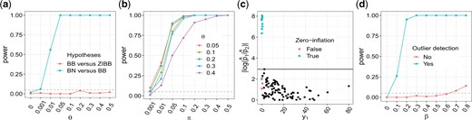
Illustration of model selection and outlier detection. (a) Hypothesis testing of BB versus ZIBB and of BN versus BB. Data were generated from the BB distribution as the over-dispersion parameter θ varied from 0 to 0.5. The dashed horizontal line indicates the nominal significance level 0.05; (b) power of the likelihood-ratio test. Data were generated from ZIBB as θ and π were both varied; (c) outlier detection. Data were generated from ZIBB with $\theta =0.1$ and $\pi =0.1$⁠. The solid black horizontal line indicates the threshold for identifying outliers; (d) the effect of outlier detection on the power. Data from two groups were generated from ZIBB with $\theta =0.1,\hspace{0.17em}\pi =0.1$ and ${\alpha }_1=0.5/\theta -0.5=4.5$ for one group and ${\alpha }_1=4.5(1+\beta )$ for the other group, as the effect size β varied

Next we compared the performance of adaANCOM and other DA testing methods. Figure 3 shows the simulation results when the generating distribution was DTM or ZIDTM with the tree and DA pattern displayed in Supplementary Figure S2. For DTM, all methods except ANCOM and edgeR had the desired precision which means they could control the false discovery rate (FDR) at 0.05. As shown in the lower panel of Figure 3a, adaANCOM and adaANCOM-S performed similarly and both were superior to others especially for moderate to large values of β. For ZIDTM, we see from Figure 3b that the overall conclusion is the same as for DTM, except that adaANCOM-S was inferior to adaANCOM. This highlights the importance of model selection in the presence of over-dispersion and zero-inflation. Supplementary Figure S3 shows that, the performance of adaANCOM deteriorated as the degree of over-dispersion increased, but it still was the best performer. The FDR of ANCOM was high because it uses the reject number among the K—1 hypotheses to decide whether or not a taxon is differentially abundant. Previous studies have found that ANCOM has an inflated FDR (Weiss et al., 2017) which is consistent with our results. One reason for the poor performance of edgeR and DESeq2 is that the underlying scaling normalization was unreliable, especially when the zero proportion was large. We note that DESeq2 may fail to provide a solution in situations with a larger proportion of zeros. The poor performance of t-test results from the compositionality and large proportion of zeros. Since the Wilcoxon rank-sum test applied directly to the raw counts, its performance was strongly affected by the sequence depth and fraction of zeros.

Fig. 3.

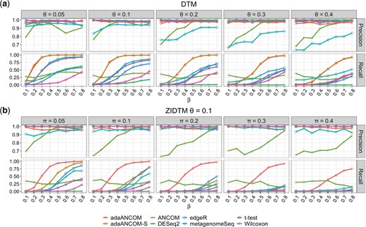
Precision and recall comparison of different DA testing methods. (a) Data were generated from DTM with varying values of dispersion parameter ${\theta }_v=\theta$ and effect size β, and with the tree and DA pattern displayed in Supplementary Figure S2; (b) data were generated from ZIDTM with varying values of zero-inflation proportion ${\pi }_v=\pi$ and a fixed dispersion ${\theta }_v=0.1$⁠, and again with the tree and DA pattern displayed in Supplementary Figure S2. The testing method in adaANCOM and adaANCOM-S was t-test

Then we explored the robustness of adaANCOM with more complex DA patterns and tree structures (Supplementary Figs S4–S12). adaANCOM was the clear overall winner. It was robust to the specification of DA pattern (Supplementary Figs S4–S9), and was insensitive to the tree size (Supplementary Figs S10–S12).

We also simulated a tree with K = 100 leaves (Supplementary Figs S13). To mimic real data, we generated data from ZIDTM using parameters learned based on the HMP dataset, as detailed in Supplementary Figure S14. On the tree, we randomly set some nodes to be differentially abundant, and highlighted three subtrees with different colors (Supplementary Figs S13). We would like to compare the results at both the whole tree and subtree levels, using either the full dataset or subsets of data corresponding to subtrees. The results are shown in Figures 4 and Supplementary Figure S15. adaANCOM had the highest recall and comparable precision, and hence the highest F1 score, across all scenarios. This type of coherence is highly desirable, as it indicates that adaANCOM is in some sense robust to tree pruning and OTU screening or preprocessing. In contrast, some methods, such as edgeR, were sensitive to the size of the OTU set, partly because of their built-in normalization processes.

Fig. 4.

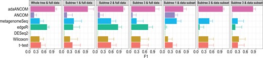
F1 score comparison of different DA testing methods. Data were generated from ZIDTM with parameters estimated based on the HMP dataset, and with the tree and DA pattern depicted in Supplementary Figure S13. ‘Whole tree’ refers to results calculated based on all leaves while ‘subtree’ refers to results summarized for leaves corresponding to each subtree, with parameters estimated using either the full data or data subsets

3.1.3 Additional simulation settings and results

It seems as if t-test and Wilcoxon rank-sum test had higher precision values than ANCOM and edgeR. This is contradictory to common sense (Mandal et al., 2015; Weiss et al., 2017). There were two reasons for the unusual behavior of t-test and Wilcoxon rank-sum test in the above simulation studies. First, for both groups the sequencing depth was generated from the same distribution. Second, simulated data were generated at each split of the tree recursively in a top-down and compositionally aware manner. To better demonstrate how t-test and Wilcoxon rank-sum test control the FDR, we explored a simple data generating mechanism as follows. We first generated the sequencing depth uniformly from 10K to 1000K for one group, and from 10K to 100K for the other group. We then generated data from DTM (or ZIDTM) with the same parameters for the two groups. Finally, we selected a subset of leaf nodes and multiplied their counts by some random effect size for one group, so that they were differentially abundant. The log effect size was drawn uniformly from –5 to 5. Note that, in this case, an increase in counts of one or more OTUs necessarily implies an increase in relative abundance of them and a concomitant decrease in relative abundance of the other OTUs and vice versa. The results are shown in Supplementary Table S1. We can see that t-test, Wilcoxon rank-sum test and edgeR had low precision across all settings, and that DESeq2, ANCOM and metagenomeSeq inflated the FDR in some cases. Again, adaANCOM and adaANCOM-S controlled the FDR better than other methods, and adaANCOM had the overall best performance.

So far, the simulated settings give advantages to adaANCOM. As suggested by a referee, we considered a new data generating mechanism by using the upcoming software SparseDOSSA 2 (https://huttenhower.sph.harvard.edu/sparsedossa2). Specifically, we simulated abundances of each taxon by SparseDOSSA 2 and aggregated them along a tree. However, since SparseDOSSA 2 requires an input count matrix for learning and setting its parameters, we used synthetic data generated from the DTM (or ZIDTM) distribution using the same tree. This makes some sense, because otherwise the tree is arbitrary and the results based on adaANCOM are not meaningful and not interpretable. The results are shown in Supplementary Figure S16. As we can see, all methods had comparable precision score, while adaANCOM got higher recall and F1. Thus, to some degree, the information aggregated from leaf nodes to internal nodes was helpful for boosting the detection power of adaANCOM. We also considered the setting in which the tree is arbitrary or misspecified, and in such a case adaANCOM did not outperform others. This is as expected, because adaANCOM is a tree-based extension of ANCOM, and when the tree is misspecified or unavailable, it is better to use ANCOM or metagenomeSeq, which are designed specifically for microbiome data.

3.2 Real data examples

3.2.1 HMP data

In this section, we applied the posterior mean transformation to the HMP data. HMP, launched in 2007, is a two-phase project aiming to facilitate characterization of the microbiota to understand the role of microbiome in human health and disease. In our analysis the data come from the first phase, in which 300 healthy individuals were recruited to investigate whether there is a core healthy microbiome. For each individual, microbial samples were collected from at most 18 different sites of human body across 3 visits, and these body sites belong to 4 major regions (oral cavity, gut, vagina and skin). The microbial samples were then sequenced at four sequencing centers (Lloyd-Price et al., 2017).

To illustrate the effect of model selection and data transformation, we extracted data from 16S rRNA sequencing of all body sites and the first two visits. We restricted attention to data processed by the Washington University Genome Center, which had the largest number of samples, to reduce the batch effect. Using the tax_glom function in the R package phyloseq, we consolidated taxa at different taxonomic levels for each body site. We also filtered samples with total reads less than 1000 and taxa with prevalence less than 20%. After data preprocessing, the sample sizes ranged from 52 to 112 and the numbers of species from 341 to 1513 (Supplementary Table S2). In addition, there was a phylogenetic tree showing the relationships among these taxa.

Before proceeding, we investigated the necessity of model selection by applying likelihood-ratio tests at each internal node to taxa abundance data separately for each body site and each visit. The results are shown in Figure 5 and Supplementary Table S3. As we can see, at the genus level the proportion of selected models being BB is the largest across all sites, indicating that taxa counts were over-dispersed, as expected. Furthermore, the proportion of ZIBB ranges from 2.63% to 41.2% and from 3.45% to 46.9% for two visits respectively, and hence model selection is essential. There is clear evidence that the composition of taxa varies widely across body sites, and that the within-individual variation is also evident but is much smaller.

Fig. 5.

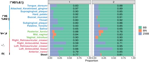
Results of model selection across the 18 body sites and two visits at the genus level. The numbers shown in each bar are the proportions of chosen models being BB

For each sample, we normalized the counts based on the posterior mean transformation, calculated the Shannon’s index and the Simpson’s index, and then compared each index between the two visits. We see that, using the Wilcoxon rank-sum test and the Bonferroni bound, there is no significant difference in alpha diversity between the two visits for all taxonomic levels (Supplementary Figs S17). We then combined the values for each index from the two visits, and compared each body site to others. From Figure 6 and Supplementary Figure S18, we can see that the alpha diversity values within the same major region was more similar to each other than those in different regions (Lloyd-Price et al., 2017).

Fig. 6.

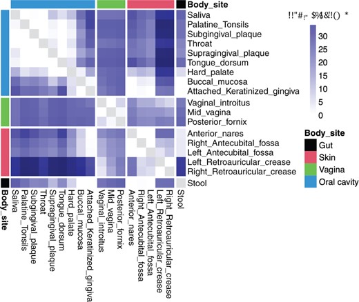
Comparing the alpha diversity between each pair of body sites at the genus level. P-values were obtained using the Wilcoxon rank-sum test and Bonferroni correction. The upper and lower triangles show the results for the Shannon’s index and the Simpson’s index, respectively

We then used the transformed stool data for DA analysis between two visits at the species level without removing the taxa with prevalence less than 20%. After pre-processing, 6965 species of 108 samples were left and the zero proportion was about 90%. The results are shown in Supplementary Table S4. Note that an error occurred for running DESeq2 to estimate the size factor. For most methods, species were not significantly differentially abundant between two visits, which was as expected and consistent with the results in Supplementary Figure S17. edgeR stood out as an exception, and species detected by it were likely false discoveries. We further carried out DA analysis between gut and other body sites at the species level. The results are summarized in Supplementary Table S5. We can see that t-test tends to detect more differentially abundant species in most cases, followed by Wilcoxon rank-sum test, and then by ANCOM and metagenomeSeq. There were some errors occurred when running DESeq2 and edgeR.

3.2.2 Gut microbiota and malnutrition

Gut microbiota play an important role in malnutrition, especially for children (Blanton et al., 2016). Using the random forest algorithm, researchers identified a set of 60 bacterial taxa at the OTU level that exhibited the highest power of predicting malnutrition for Bangladeshi children (Subramanian et al., 2014). In this section, we revisited this dataset and applied adaANCOM and other methods to detect DA taxa between healthy and malnourished children. Following Liu et al. (2020), we built a phylogenetic tree using representative sequences for the 60 taxa (Supplementary Figure S19), and treated the relative importance of these taxa assessed by random forest as the gold standard.

We focused on the 22 normal and 40 malnutrition subjects, all aged from 12 to 18 months. As in Subramanian et al. (2014), we rarefied the 62 samples to the lowest depth by the rarefy function in the R package GUniFrac. To evaluate the performance of a DA testing method, for each $t\in \{5,10,15,20,25\}$⁠, we calculated the F1 score, $F1(t)$⁠, by comparing the t taxa having the smallest P-values with the top-t taxa ranked by random forest. The results are shown in Figure 7. We can see that adaANCOM performed well overall.

Fig. 7.

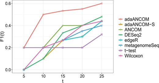
F1 score comparison of different DA testing methods, as we varied the number t of top-ranked taxa by random forest

We then compared the DA testing results for adaANCOM and those for its competitors on the tree. Since all the 60 taxa were predictive of the malnutrition status, the larger the number of identified taxa, the better the DA testing method. adaANCOM detected a total of 38 taxa, of which 21 were unique. Supplementary Figure S20 shows a tree-based visualization of the outcomes. We can see that differentially abundant taxa identified by our method tend to be more similarly related to each other. For example, the most significant taxon found exclusively by adaANCOM, OTU 189827 (Rumicnococcus_sp_5_1_39BFAA, P-value=$3.54\times {10}^{-15}$⁠), was ranked the second by random forest, and its sibling, OTU 364234, was also significant (Rumicnococcus_sp_5_1_39BFAA, P-value=$2.62\times {10}^{-13}$⁠) and ranked the 10th by random forest. The species Rumicnococcus_sp_5_1_39BFAA was discovered to be depleted in malnourished children (Million et al., 2017). OTU 48207 (Dialister, P-value=$2.66\times {10}^{-4}$⁠) and its slibling OTU 259261 (Megamonas, P-value=$4.14\times {10}^{-5}$⁠) were also uniquely identified by adaANCOM. The genus Dialister was experimentally verified to be positively correlated to severity of functional intestinal disorders, which are frequently observed in malnourished patients with anorexia nervosa (Mouna et al., 2019), and the genus Megamonas was shown to be more abundant in malnourished children than in healthy children (Subramanian et al., 2014).

4 Discussion

In the first part of the article, we proposed an extension of DTM, called ZIDTM, for modeling microbial abundance data. By definition, the probability mass function of ZIDTM is the product of probability mass functions of ZIDMs that factorize over the tree. To our knowledge, ZIDTM is the most flexible multivariate distribution for count data that simultaneously takes into account over-dispersion, data sparsity, complex inter-taxon dependencies and phylogenetic structure among taxa. We developed an expectation-maximization algorithm for maximum likelihood estimation, which can be implemented efficiently on a parallel architecture computer. To address the matching problem, for each internal node and each possible ordering of its child nodes, a separate ZIDM model is fitted and the best-fitting model is selected. Incorporating the phylogeny greatly alleviates the matching problem of GDM and ZIDM in high dimensions. To further address the compositionality problem, we proposed an empirical Bayes approach to transform microbial counts into non-zero relative abundances, by plugging the maximum likelihood estimates under ZIDTM into the posterior mean. To improve the quality of posterior mean transformation, at each internal node, model selection is conducted based on a two-stage likelihood-ratio test. It is worth noting that ZIDTM also allows one to study the effects of covariates, such as dietary nutrients on microbial composition, although computational tractability is a concern when both the number of covariates and the number of taxa are large. One limitation of ZIDTM is the conditional independence assumption across internal nodes. It is interesting and important to relax this assumption. Work along this line is in progress.

In the second part, using the posterior-mean-transformed data (that is, estimated compositions), we proposed an extension of ANCOM, called adaANCOM, for DA testing. adaANCOM consists of two steps. First, it tests the hypotheses at the internal node level. Then, based on the results in the first step, it builds log-ratios adaptively on the tree for each leaf node, and tests for DA for the corresponding taxon. To prevent log-ratios from taking abnormal values, an additional step of outlier detection is conducted. adaANCOM greatly reduces the computational complexity of ANCOM in high dimensions from $O(|\mathcal{L}{|}^2)$ to $O(|\mathcal{L}|)$⁠, controls the false discovery rate better than ANCOM, and allows for a tree-based visualization of the results. Our work connects to the recent interest in phylogenetically informed analysis of microbiome data. However, as mentioned previously, most of the phylogeny-aware testing procedures concern the overall significance of the association between the microbiome and an outcome variable. For example, the phylogenetic tree-based microbiome association test of Kim et al. (2020) is also composed of two steps, with the same first step as that of adaANCOM. However, the results in the first step are combined in the second step to carry out a global association test, rather than testing associations with each individual taxon. We have implemented our methodology in the R package adaANCOM, and demonstrated its good performance using extensive simulation studies and two real data applications. adaANCOM implicitly assumes that data are generated at each split of the tree recursively in a top-down manner. However, there are situations in which this assumption could be violated. Extensions of adaANCOM to handle top-down, bottom-up or mixed cases would be an interesting area for future research.

Acknowledgements

The authors thank Yaru Song and Tiantian Liu for their valuable feedback on methodology and real data analysis. Chao Zhou would also like to thank the China Scholarship Council (CSC) for supporting his study at Yale School of Public Health.

Funding

This research was supported in part by the National Key R&D Program of China [2018YFC0910500], National Natural Science Foundation of China [11971017], Shanghai Municipal Science and Technology Major Project [2017SHZDZX01], Multidisciplinary Cross Research Foundation of Shanghai Jiao Tong University [YG2019QNA26, YG2019QNA37, YG2021QN06] and Neil Shen’s SJTU Medical Research Fund.

Conflict of Interest: none declared.