A fast data-driven method for genotype imputation, phasing and local ancestry inference: MendelImpute.jl

Abstract

Motivation

Current methods for genotype imputation and phasing exploit the volume of data in haplotype reference panels and rely on hidden Markov models (HMMs). Existing programs all have essentially the same imputation accuracy, are computationally intensive and generally require prephasing the typed markers.

Results

We introduce a novel data-mining method for genotype imputation and phasing that substitutes highly efficient linear algebra routines for HMM calculations. This strategy, embodied in our Julia program MendelImpute.jl, avoids explicit assumptions about recombination and population structure while delivering similar prediction accuracy, better memory usage and an order of magnitude or better run-times compared to the fastest competing method. MendelImpute operates on both dosage data and unphased genotype data and simultaneously imputes missing genotypes and phase at both the typed and untyped SNPs (single nucleotide polymorphisms). Finally, MendelImpute naturally extends to global and local ancestry estimation and lends itself to new strategies for data compression and hence faster data transport and sharing.

Availability and implementation

Software, documentation and scripts to reproduce our results are available from https://github.com/OpenMendel/MendelImpute.jl.

Supplementary information

Supplementary data are available at Bioinformatics online.

1 Introduction

Haplotyping (phasing) is the process of inferring unobserved haplotypes from observed genotypes. It is possible to deduce phase from the observed genotypes of surrounding pedigree members (Sobel et al., 1996), but pedigree data are no longer considered competitive with linkage disequilibrium data. Current methods for phasing and genotype imputation exploit public reference panels such as those curated by the Haplotype Reference Consortium (HRC) (McCarthy et al., 2016) and the NHLBI TOPMed Program (Taliun et al., 2021). The sizes of these reference panels keep expanding: from 1000 samples in 2012 (1000 Genomes Project Consortium et al., 2012), to about 30 000 in 2016 (McCarthy et al., 2016), to over 90 000 in 2019 (Taliun et al., 2021). Genome-wide association studies (GWAS), the primary consumers of imputation, exhibit similar trends in increasing sample sizes and denser SNP typing (Sudlow et al., 2015). Despite these technological improvements, phasing and imputation methods are still largely based on hidden Markov models (HMMs). Through decades of successive improvements, HMM software is now >10 000 times faster than the original software (Das et al., 2018), but the core HMM principles remain relatively unchanged. This paper explores an attractive data-driven alternative for imputation and phasing that is faster and simpler than HMM methods.

HMMs capture the linkage disequilibrium in haplotype reference panels based on the probabilistic model of Li and Stephens (2003). The latest HMM software programs include Minimac 4 (Das et al., 2016), Beagle 5 (Browning et al., 2018) and Impute 5 (Rubinacci et al., 2020). These HMM programs all have essentially the same imputation accuracy (Browning et al., 2018), are computationally intensive and generally require prephased genotypes. The biggest computational bottleneck facing these programs is the size of the HMM state space. An initial prephasing (imputation) step fills in missing phases and genotypes at the typed markers in a study. The easier second step constructs haplotypes on the entire set of SNPs in the reference panel from the prephased data (Howie et al., 2012). This separation of tasks forces users to chain together different computer programs, reduces imputation accuracy (Das et al., 2018) and tends to inflate overall run-times even when the individual components are well optimized.

Purely data-driven techniques are potential competitors to HMMs in genotype imputation and haplotyping. Big data techniques replace massive amounts of training data with detailed models for prediction. This substitution can reduce computation times and, if the data are incompatible with the assumptions underlying the HMM, improve accuracy. Haplotyping HMMs, despite their appeal and empirically satisfying error rates, make simplifying assumptions about recombination hot spots and linkage patterns. We have previously demonstrated the virtues of big data methods in genotype imputation with haplotyping (Chen et al., 2012) and without haplotyping (Chi et al., 2013). SparRec (Jiang et al., 2016) refines the latter method by adding additional information on matrix coclustering. These two matrix completion methods efficiently impute missing entries via low-rank approximations. Unfortunately, they also rely on computationally intensive cross validation to find the optimal rank of the approximating matrices. On the upside, matrix completion circumvents prephasing, exploits reference panels and readily imputes dosage data, where genotype entries span the entire interval [0,2].

Despite these advantages, data-driven methods have not been widely accepted as alternatives to HMM methods. Although possible in principle, our previous program (Chi et al., 2013) did not build a pipeline to handle large reference panels. Here, we introduce a novel data-driven method to fill this gap. Our software MendelImpute (a) avoids the prephasing step, (b) exploits known haplotype reference panels, (c) supports dosage data, (d) runs extremely fast, (e) makes a relatively small demand on memory and (f) naturally extends to local and global ancestry inference. Its imputation error rate is slightly higher than the best HMM software but still within a desirable range. MendelImpute is open source and forms a part of the OpenMendel platform (Zhou et al., 2020), which is written in the modern Julia programming language (Bezanson et al., 2017). We demonstrate that MendelImpute is capable of dealing with HRC data even on a standard laptop. In coordination with our packages VCFTools.jl for VCF files, SnpArrays.jl for PLINK files and BGEN.jl for BGEN files, OpenMendel powers a streamlined pipeline for end-to-end data analysis.

For each chromosome of a study subject, MendelImpute reconstructs two extended haplotypes ${\mathbf{E}}_1$ and ${\mathbf{E}}_2$ that cover the entire chromosome. Both ${\mathbf{E}}_1$ and ${\mathbf{E}}_2$ are mosaics of reference haplotypes with a few break points where a switch occurs from one reference haplotype to another. The break points presumably represent contemporary or ancient recombination events. MendelImpute finds these reference segments and their break points. From ${\mathbf{E}}_1$ and ${\mathbf{E}}_2$⁠, it is trivial to impute missing genotypes, both typed and untyped. The extended haplotypes can be painted with colors indicating the region on the globe from which each reference segment was drawn. The number of SNPs assigned to each color immediately determine ethnic proportions and plays into admixture mapping. The extended segments also serve as a convenient device for data compression. One simply stores the break points and the index of the reference haplotype assigned to each segment. Finally, ${\mathbf{E}}_1$ and ${\mathbf{E}}_2$ can be nominated as maternal or paternal whenever either parent of a sample subject is also genotyped.

2 Materials and methods

Our overall imputation strategy operates on an input matrix $\mathbf{X}$ whose columns are sample genotypes at the typed markers. The entries of $\mathbf{X}$ represent alternate allele counts $x_{ij}\in [0,2]\cup \left\{\text{missing}\right\}$⁠. The reference haplotypes are stored in a matrix $\mathbf{H}$ whose columns are haplotype vectors with entries $h_{ij}\in \{0,1\}$⁠, representing reference and alternative alleles, respectively. Given these data, the idea is to partition each sample’s genotype vector into small adjacent genomic windows. In each window, many reference haplotypes collapse to the same unique haplotype at the typed SNPs. We find the two unique haplotypes whose vector sum best matches the sample genotype vector. Then we expand the unique haplotypes into two sets of matching full haplotypes and intersect these sets across adjacent windows. Linkage disequilibrium favors long stretches of single reference haplotypes punctuated by break points. Our strategy is summarized in Figure 1. A detailed commentary on the interacting tactics appears in subsequent sections.

Fig. 1.

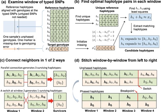
Overview of MendelImpute’s algorithm. (a) After alignment, imputation and phasing are carried out on short, nonoverlapping windows of the typed SNPs. (b) Based on a least squares criterion, we find two unique haplotypes whose vector sum approximates the genotype vector on the current window. Once this is done, all reference haplotypes corresponding to these two unique haplotypes are assembled into two sets of candidate haplotypes. (c) We intersect candidate haplotype sets window by window, carrying along the surviving set and switching orientations if that result generates more surviving haplotypes. (d) After three windows, the top extended chromosome possesses no surviving haplotypes, but a switch to the second orientation in the current window allows ${\mathbf{h}}_5$ to survive on the top chromosome. Eventually, we must search for a break point separating ${\mathbf{h}}_1$ from ${\mathbf{h}}_2$ or ${\mathbf{h}}_6$ between windows 3 and 4 (bottom panel).

2.1 Missing data in typed and untyped SNPs

There are two kinds of missing data requiring imputation. A GWAS dataset may sample on the order of 10⁶ SNPs across the genome. We call SNPs that are sampled at this stage typed SNPs. Raw data from a GWAS study may contain entries missing at random due to experimental errors, but the missing rate is usually low, at most a few percent, and existing programs (Loh et al., 2016) usually impute these in the prephasing step. When modern geneticists speak of imputation, they refer to imputing phased genotypes at the unsampled SNPs present in the reference panel. We call the unsampled markers untyped SNPs. The latest reference panels contain from 10⁷ to 10⁸ SNPs, so an imputation problem can have >90% missing data. We assume that the typed SNPs sufficiently cover the entire genome. From the mosaic of typed and untyped SNPs, one can exploit local linkage disequilibrium to infer for each person his/her phased genotypes at all SNPs, typed and untyped. As a first step one must situate the typed SNPs among the ordered SNPs in the reference panel (see Fig. 1a). The Julia command indexin() quickly finds the proper alignment.

2.2 Finding optimal haplotype pairs via least squares

Suppose there are d unique haplotypes ${\mathbf{h}}_1,\dots ,{\mathbf{h}}_d$ (with entries 0 or 1) in a genomic window (see Fig. 1b), where the Supplementary Material discusses how to efficiently compute them. Consider a genotype vector $\mathbf{x}$ with entries $x_i\in [0,2]\cup \left\{\text{missing}\right\}$⁠. The goal is to find the two unique haplotypes ${\mathbf{h}}_i$ and ${\mathbf{h}}_j$ such that $\mathbf{x}\approx {\mathbf{h}}_i+{\mathbf{h}}_j$⁠. The best haplotype pair is selected by minimizing the least squares criterion

$$\begin{array}{c}\left|\right|\mathbf{x}-{\mathbf{h}}_i-{\mathbf{h}}_j|{|}_2^2\hspace{0.17em}=\left|\right|\mathbf{x}|{|}_2^2+|\left|{\mathbf{h}}_i\right|{|}_2^2+\left|\right|{\mathbf{h}}_j|{|}_2^2+2{\mathbf{h}}_i^T{\mathbf{h}}_j\hfill \\ \\ \hfill & -2{\mathbf{x}}^T{\mathbf{h}}_i-2{\mathbf{x}}^T{\mathbf{h}}_j\hfill \end{array}$$

(1)

over all $\left(\begin{array}{c}d\\ 2\end{array}\right)+d$ haplotype combinations. To fill in a missing value x_i, we naively initialize it with the mean at each typed SNP. This action may lead to imputation errors when the typed SNPs exhibit a large proportion of missing values. We discuss a strategy to remedy this bias in the Supplementary Material.

To minimize criterion (1) efficiently, suppose the genotype vectors ${\mathbf{x}}_i$ constitute the columns of a genotype matrix X, and suppose the haplotype vectors ${\mathbf{h}}_i$ constitute the columns of a haplotype matrix H. Given these conventions we recover all inner products ${\mathbf{x}}_i^T{\mathbf{h}}_j$ and ${\mathbf{h}}_i^T{\mathbf{h}}_j$ in Equation (1) as entries of two matrix products; the two corresponding BLAS (Basic Linear Algebra Subroutines) (Lawson et al., 1979) level-3 calls produce

$$\begin{array}{cc}{\mathbf{X}}^T\mathbf{H}\hfill & ={\left(\begin{array}{ccc}{\mathbf{x}}_1^T{\mathbf{h}}_1& \cdots & {\mathbf{x}}_1^T{\mathbf{h}}_d\\ ⋮& & ⋮\\ {\mathbf{x}}_n^T{\mathbf{h}}_1& \cdots & {\mathbf{x}}_n^T{\mathbf{h}}_d\end{array}\right)}_{n\times d}\hfill \\ {\mathbf{H}}^T\mathbf{H}\hfill & ={\left(\begin{array}{ccc}\left|\right|{\mathbf{h}}_1|{|}_2^2& \cdots & {\mathbf{h}}_1^T{\mathbf{h}}_d\\ ⋮& & ⋮\\ {\mathbf{h}}_d^T{\mathbf{h}}_1& \cdots & \left|\right|{\mathbf{h}}_d|{|}_2^2\end{array}\right)}_{d\times d}\hfill \end{array}$$

(2)

.

These allow one to quickly assemble a matrix $\mathbf{M}$ with entries $m_{ij}=\left|\right|{\mathbf{h}}_i|{|}_2^2+|\left|{\mathbf{h}}_j\right|{|}_2^2+2{\mathbf{h}}_i^T{\mathbf{h}}_j$ and for each sample ${\mathbf{x}}_k$ a matrix $\mathbf{N}$ with entries $n_{ij}=-2{\mathbf{x}}_k^T{\mathbf{h}}_i-2{\mathbf{x}}_k^T{\mathbf{h}}_j$⁠. Therefore, to find the best haplotype pair $({\mathbf{h}}_i,{\mathbf{h}}_j)$ for the sample ${\mathbf{x}}_k$⁠, we search for the minimum entry $m_{ij}+n_{ij}$ of the d × d matrix $\mathbf{M}+\mathbf{N}$ across all indices $i\ge j$⁠. Extremely unlikely ties are arbitrarily broken. Note that the constant term $\left|\right|{\mathbf{x}}_k|{|}_2^2$ can be safely ignored in optimization. Data import and this minimum entry search are the computational bottlenecks of our software. Once such a haplotype pair is identified, all reference haplotype pairs identical to $({\mathbf{h}}_i,{\mathbf{h}}_j)$ in the current window give the same optimal ${\ell }_2$ error.

2.3 Phasing by intersecting haplotype sets

As just described, each window w along a sample chromosome generates an optimal pair of unique haplotypes. These expand into two sets $S_{w1}$ and $S_{w2}$ of reference haplotypes (see Fig. 1b). In the first window, we arbitrarily assign S₁₁ to extended haplotype 1 and S₁₂ to extended haplotype 2. From here on the goal is to reconstruct two extended composite haplotypes ${\mathbf{E}}_1$ and ${\mathbf{E}}_2$ that cover the entire chromosome. Let w index the current window. The two sets $S_{w-1,1}$ and $S_{w-1,2}$ are already phased. The new sets $S_{w1}$ and $S_{w2}$ are not, and their phases must be resolved and their entries pruned by intersection to achieve extended haplotype parsimony. The better orientation is one which generates more surviving haplotypes after intersection (see Fig. 1c). Here, we count surviving haplotypes across both sets of orientation. The better orientation and the corresponding survivor sets are propagated to subsequent windows. If either intersection is empty at window w, then a break is declared, the empty set is replaced by the entire haplotype set of window w, and a new reference segment commences (see Fig. 1d). Ties and double empties virtually never occur. Repeated intersection may fail to produce singleton haplotype sets, in which case we randomly designate a winner to use for breakpoint search.

For example, suppose $S_{11}=\{{\mathbf{h}}_1,{\mathbf{h}}_2,{\mathbf{h}}_3\}$ and $S_{12}=\{{\mathbf{h}}_4,{\mathbf{h}}_5,{\mathbf{h}}_6\}$ are the (arbitrarily) phased sets in window 1. Since window 2 is not yet phased, the two sets $S_{21}=\{{\mathbf{h}}_1,{\mathbf{h}}_2,{\mathbf{h}}_6\}$ and $S_{22}=\{{\mathbf{h}}_5,{\mathbf{h}}_7,{\mathbf{h}}_8\}$ can be assigned to extended haplotypes 1 and 2, respectively, or vice versa as depicted in Figure 1c. The first orientation is preferred since it generates three surviving haplotypes $\{{\mathbf{h}}_1,{\mathbf{h}}_2\}$ and $\left\{{\mathbf{h}}_5\right\}$ bridging windows 1 and 2. Thus, $\{{\mathbf{h}}_1,{\mathbf{h}}_2\}$ and $\left\{{\mathbf{h}}_5\right\}$ are assigned at window 2 with this orientation and propagated to window 3. In window 3, the contending pairs are $\{{\mathbf{h}}_1,{\mathbf{h}}_2\}\cap \{{\mathbf{h}}_1,{\mathbf{h}}_3\}$ and $\left\{{\mathbf{h}}_5\right\}\cap \{{\mathbf{h}}_5,{\mathbf{h}}_7\}$ versus $\{{\mathbf{h}}_1,{\mathbf{h}}_2\}\cap \{{\mathbf{h}}_5,{\mathbf{h}}_7\}$ and $\left\{{\mathbf{h}}_5\right\}\cap \{{\mathbf{h}}_1,{\mathbf{h}}_3\}$⁠. The former prevails, and $\left\{{\mathbf{h}}_1\right\}$ and $\left\{{\mathbf{h}}_5\right\}$ are assigned to window 3 and propagated to window 4. In window 4, the opposite orientation is preferred (see Fig. 1d). In this empty intersection case, we set $S_{41}=\{{\mathbf{h}}_2,{\mathbf{h}}_6\}$ and $S_{42}=\left\{{\mathbf{h}}_5\right\}$ and continue the process. Later we return and resolve the breakpoint in extended haplotype 1 between windows 3 and 4.

2.4 Resolving breakpoints

The unique haplotype pairs found for adjacent windows are sometimes inconsistent and yield empty intersections. In such situations, we search for a good break point. Figure 1d illustrates a single-breakpoint search. In this example, we slide the putative break point b across windows 3 and 4 in the top extended haplotype to minimize the least squares value determined by the observed genotype, ${\mathbf{h}}_5$ spanning both windows, and the breakpoint b between ${\mathbf{h}}_1$ and ${\mathbf{h}}_2\cup {\mathbf{h}}_6$⁠. When there is a double mismatch, we must search for a pair (b₁, b₂) of breakpoints, one for each extended haplotype. The optimal pair can be determined by minimizing the least squares distances generated by all possible breakpoint pairs (b₁, b₂). Thus, double breakpoint searches scale as a quadratic. Fortunately, under the adaptive window width strategy described in the Supplementary Material, the number of typed SNPs in each window typically is on the order of 10². In this range, quadratic search remains efficient.

2.5 Imputation and phasing of untyped SNPs

Once haplotyping is complete, it is trivial to impute missing SNPs. Each missing SNP is located on the reference map, and its genotype is imputed as the sum of the alleles on the extended haplotypes ${\mathbf{E}}_1$ and ${\mathbf{E}}_2$⁠. Observed genotypes are untouched unless the user prefers phased genotypes. In this case MendelImpute will override observed genotypes with phased haplotypes similar to Minimac 4. Unfortunately, MendelImpute cannot compute estimated dosages. As shown in Section 3.4 on alternative compression schemes, the extended haplotypes ${\mathbf{E}}_1$ and ${\mathbf{E}}_2$ can be output rather than imputed genotypes at the user’s discretion.

2.6 Compressed reference panels

Large reference files are typically stored as compressed VCF files. Since VCF files are plain text files, they are large and slow to read. Read times can be improved by computing and storing an additional tabix index file (Li, 2011), but file size remains a problem. Consequently, every modern imputation program has developed its own specialized reference file format (for instance, the m3vcf, imp5 and bref3 formats of Minimac, Impute and Beagle, respectively) for improving read times and storage efficiency. We propose yet another compressed format for this purpose: the jlso format, and we compare it against other formats in Table 1. Details for generating the jlso format are discussed in the Supplementary Material.

Table 1.

Storage size required for various compressed reference haplotype formats

Dataset	Size (MB) for format:
	vcf.gz	jlso	bref3	m3vcf.gz	imp5
sim 10K	49	6	18	7	57
sim 100K	472	56	81	29	565
sim 1M	4660	776	415	NA	5650
1000G chr10	459	188	342	116	621
1000G chr20	200	89	154	52	279
HRC chr 10	3346	1328	1156	529	3636
HRC chr 20	1510	706	554	253	1610

Note: Here, vcf.gz is the standard compressed VCF format; jlso is used by MendelImpute; bref3 is used by Beagle 5.1; m3vcf.gz is used by Minimac 4; and imp5 is used by Impute 5. For all jlso files, we chose the maximum number of unique haplotypes per window to be $d_{\text{max}}=1000$⁠. Note we could not generate the m3vcf.gz file for the sim 1 M panel because it required too much memory (RAM).

2.7 Real and simulated data experiments

For each dataset, we use only biallelic SNPs. Table 2 summarizes the real and simulated data used in our comparisons.

Table 2.

Summary of real and simulated datasets used in our experiments

Dataset	Total SNP	Typed SNP	Sample	Ref Haps	Miss %
Sim 10K	62 704	22 879	1000	10 000	0.5
Sim 100K	80 029	23 594	1000	100 000	0.5
Sim 1M	97 750	23 092	1000	1 000 000	0.5
1000G chr10	3 968 020	192 683	52	4904	0.1
1000G chr20	1 802 261	96 083	52	4904	0.1
HRC chr10	1 809 068	191 210	1000	52 330	0.1
HRC chr20	829 265	95 414	1000	52 330	0.1

Note: For the 1000G and HRC datasets, the SNPs also present on the Infinium Omni5-4 Kit constitute the typed SNPs. Miss % is the percentage of typed SNPs randomly masked to mimic random missing data. For ancestry estimation, we used the top 50 000 most ancestry informative SNPs in each 1000G chromosome.

2.7.1 Simulated data

To test scalability across a broad range of panel sizes, we simulated three 10 Mb sequence datasets with 12 000, 102 000 and 1 002 000 haplotypes using the software msprime (Kelleher et al., 2016). We randomly selected 1000 samples (2000 haplotypes) from each pool to form the target genotypes and used the remaining to form the reference panels. The SNPs with minor allele frequency greater than 5% were designated the typed SNPs. Approximately 0.5% of the typed genotypes were randomly masked to introduce missing values.

2.7.2 1000 Genomes Data

We downloaded the publicly available 1000 Genomes (1000G) phase 3 dataset (1000 Genomes Project Consortium et al., 2015, 2012) from Beagle’s website (Browning et al., 2018). The original 1000 Genomes dataset contains 2504 samples with 49 143 605 phased genotypes across 26 different populations, as summarized in the Supplementary Material. In our study, structural variants and markers with <5 copies of the minor allele present in the data or with nonunique identifiers were excluded. We focused on chromosomes 10 and 20 in our speed and accuracy experiments. Following (Browning et al., 2018; Rubinacci et al., 2020), we randomly selected two samples from each of the 26 populations to serve as imputation targets. All other samples became the reference panel. We chose SNPs present on the Infinium Omni5-4 Kit to be typed SNPs and randomly masked 0.1% of the typed genotypes to mimic data missing at random.

For ancestry inference experiments, on each chromosome, we chose the top 50 000 most ancestry informative markers (AIMs) with minor allele frequency $\ge 0.01$ as the typed SNPs (Brown and Pasaniuc, 2014). The AIM markers were computed using VCFTools.jl. Samples from ACB, ASW, CLM, MXL, PEL and PUR (African Caribbeans, Americans of African Ancestry, Colombians, Mexican Ancestry, Peruvians and Puerto Ricans, respectively; total n = 504) are assumed admixed and employed in admixture experiments. Samples from the 20 remaining populations (total n = 2000) are assumed to exhibit less continental-scale admixture and serve as the reference panel. Unfortunately, the indigenous Amerindian populations are not surveyed in the 1000 Genomes data, so we use East Asian (EAS) and South Asian (SAS) populations as the best available proxy.

2.7.3 HRC data

We also downloaded the HRC v1.1 data from the European Genotype-Phenome archive (Lappalainen et al., 2015) (data accession = EGAD00001002729). This dataset consists of 39 741 659 SNPs in 27 165 individuals of predominantly European ancestry. We randomly selected 1000 samples in chromosomes 10 and 20 to serve as imputation targets and the remaining to serve as the reference panel. SNPs also present on the Infinium Omni5-4 Kit are chosen to be typed SNPs. Finally, we randomly masked 0.1% of the typed genotypes to mimic data missing at random.

3 Result

Due to Julia’s flexibility, MendelImpute runs on Windows, Mac and Linux operating systems, equipped with either Intel or ARM hardware.

3.1 Comparison setup

All programs were run under Linux CentOS 7 and within 10 cores of an Intel i9 9920X 3.5 GHz CPU with access to 64 GB of RAM. All reference files were previously converted to the corresponding compressed formats, bref3, m3vcf, imp5 or jlso. All target genotypes were unphased, and 0.1% or 0.5% of typed genotypes were deleted at random. Since Minimac 4 and Impute 5 required prephased data, we used Beagle 5.1’s built-in prephasing routine and report its run-time and RAM usage beside the usage statistics of the main program. All output genotypes are phased and complete.

MendelImpute was run using Julia v1.5.0. The maximum number of unique haplotypes per window (see Supplementary Material on jlso compression) was set to $d_{\text{max}}=1000$⁠, and the number of BLAS threads was set to 1 to avoid over-subscription. Beagle and Minimac were run under their default settings. Impute 5 was run on 20 Mb chunks corresponding to different chromosome regions, except for chromosome 10 of HRC. Chunks were initialized in parallel and imputed separately. Each chunk potentially employs multithreading. We used as many threads as possible without exceeding 10 total threads over all chunks. For chromosome 10 of HRC, we imputed 10 Mb chunks, with a maximum of 8 processes active at any given time. Using the maximum 10 processes or employing longer chunks resulted in out-of-memory errors.

3.2 Speed, accuracy and peak memory demand

Table 3 compares the speed, raw imputation accuracy and peak memory (RAM) usage of MendelImpute, Beagle 5.1, Impute 5 v1.1.4 and Minimac 4. Following the earlier studies (Browning et al., 2018; Das et al., 2016; Rubinacci et al., 2020), Figure 2 additionally plots the squared Pearson correlation r² between the vector of genotypes and the vector of imputed posterior genotype dosages. Note that we binned imputed minor alleles according to the minor allele count in the reference panel. For MendelImpute, we plot squared correlation r² between true genotypes and the imputed genotypes. Memory was measured via the usr/bin/time command, except for Impute 5 where memory is monitored manually via the htop command.

Fig. 2.

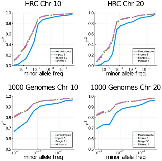
Imputation accuracy for imputed genotypes of the 1000 Genomes Project and the Haplotype Reference Consortium. Imputed alleles are binned according to minor allele frequency in the reference panel.

Table 3.

Error, time and memory comparisons on real and simulated data

	Error rate	Time (s)	Memory (GB)
Sim 10K
MendelImpute	3.00E−04	10	1.6
Impute 5	2.82E−05	43	8.9 [6.6]
Beagle 5.1	2.81E−05	189	8.8
Minimac 4	2.38E−05	271 [177]	1.0 [6.6]
Sim 100K
MendelImpute	2.19E−05	14	1.6
Impute 5	9.36E−06	43 [177]	9.9 [14.5]
Beagle 5.1	8.22E−06	279	20.1
Minimac 4	7.91E−06	3032 [253]	2.6 [14.5]
Sim 1M
MendelImpute	2.21E−05	27	4.4
Impute 5	1.33E−05	153 [752]	12.6 [25.6]
Beagle 5.1	7.01E−06	769	25.6
Minimac 4	NA	NA	NA
1000G chr10
MendelImpute	7.52E−03	34	4.1
Impute 5	4.79E−04	35 [151]	5.6 [7.3]
Beagle 5.1	4.82E−04	178	26.2
Minimac 4	4.89E−04	298 [151]	3.8 [7.3]
1000G chr20
MendelImpute	7.49E−03	14	2.2
Impute 5	4.48E−03	21 [74]	5.5 [5.3]
Beagle 5.1	4.53E−03	88	6.4
Minimac 4	4.48E−03	243 [74]	2.8 [5.3]
HRC chr10
MendelImpute	1.70E−03	183	8.4
Impute 5	8.00E−04	754 [2619]	47.6 [13.0]
Beagle 5.1	8.34E−04	3191	33.2
Minimac 4	8.57E−04	17 100 [2619]	11.5 [13.0]
HRC chr20
MendelImpute	1.89E−03	84	5.1
Impute 5	8.57E−04	645 [1319]	39.0 [13.3]
Beagle 5.1	9.10E−04	1549	22.1
Minimac 4	9.18E−04	8640 [1319]	15.1 [13.3]

Note: The best number in each cell is bold faced. The displayed error rate is the proportion of incorrectly imputed genotypes. Minimac 4 and Impute 5’s runs use the results of a prephasing step done by Beagle 5.1, whose time and memory usage are reported in brackets. For the sim 1M data, the m3vcf reference panel required for Minimac could not be computed due to excessive memory requirements.

On HRC, MendelImpute runs 18–23 times faster than Impute 5 (including prephasing time), 17–18 times faster than Beagle 5.1 and 108–119 times faster than Minimac 4. On the smaller 1000 Genomes dataset, MendelImpute runs 5–7 times faster than Impute 5, 5–6 times faster than Beagle 5.1 and 10–23 times faster than Minimac 4. Increasing the reference panel size by a factor of 100 on simulated data only increases MendelImpute’s computation time by a factor of at most three. MendelImpute also scales better than HMM methods as the number of typed SNPs increases. This improvement is evident from the timing results for simulated and real data. Thus, denser SNP arrays may benefit disproportionately from using MendelImpute. The 1000 Genomes dataset is exceptional in that it has fewer than 5000 reference haplotypes. Therefore, traversing that HMM state space is not much slower than performing the corresponding linear algebra calculations in MendelImpute. Notably, except for the HRC panels, MendelImpute spends at least 50% of its total compute time in the mundane task of simply importing the data.

In terms of error rate, MendelImpute is 1.5–1.7 times worse on 1000 Genomes data and 2.1–2.2 worse on the HRC data compared to the best HMM method. This translates to slightly lower r² values, particularly for rare alleles. On simulated data, our error rate is 2.7–10 times worse. Note the 1000 Genomes data have higher aggregate r² because the panel have undergone quality control procedures. The error rates of Impute 5, Beagle 5.1 and Minimac 4 are all similar, consistent with previous findings (Rubinacci et al., 2020). As discussed in the Supplementary Material, it is possible to improve MendelImpute’s error rate by computationally intensive strategies such as phasing by dynamic programming.

Finally, MendelImpute requires much less memory for most datasets. As explained in the methods section and the Supplementary Material, the genotype matrix and compressed reference panel are compactly represented in memory. Since most analysis is conducted in individual windows, only small sections of these matrices need to be decompressed into single-precision arrays at any one time. Consequently, MendelImpute uses at most 8.4 GB of RAM in each of these experiments. In general, MendelImpute permits standard laptops to conduct imputation even with the sizable HRC panels.

3.3 Ancestry inference for admixed populations

MendelImpute lends itself to chromosome painting, the process of coloring each haplotype segment by the country, region or ethnicity of the reference individual assigned to the segment. For chromosome painting to be of the most value, reference samples should be representative of distinct populations. Within a reference population, there should be little admixture. Also, the colors assigned to different regions should be coordinated by physical, historical and ethnic proximity. The overall proportions of the colors assigned to an individual’s genome immediately translate into global admixture coefficients. Here, we illustrate chromosome painting using chromosome 18 data from the 1000 Genomes Project. The much larger HRC data would be better suited for chromosome painting, but unfortunately its repository does not list country of origin. Our examples should therefore be considered simply as a proof of principle. As already mentioned, the populations present in the 1000 Genomes Project data are summarized in the Supplementary Material.

Figure 3a displays the painted chromosomes 18 of a native Puerto Rican (PUR, sample 1), a Peruvian from Lima, Peru (PEL, sample 2) and a person of African ancestry from the Southwest USA (ASW, sample 3). Here, a total of 20 reference populations potentially contribute genetic segments. They are colored with brown, red, blue or green to capture South Asian, East Asian, European or African backgrounds, respectively. Note that the samples from South and East Asian populations serve as a proxy for Amerindian ancestral populations. After coloring, the two PUR extended haplotypes are predominantly blue, the two PEL haplotypes are predominantly red/brown and blue, while the two ASW haplotypes are predominantly green. Interestingly, one of the PUR and one of the PEL haplotypes contain a block of African origin as well as blocks of Asian and European origin, while the ASW haplotypes contain two blocks of European origin. The relatively long blocks are suggestive of recent admixture. The resulting chromosome barcodes vividly display population origins and suggest the locations of ancient or contemporary recombination events.

Fig. 3.

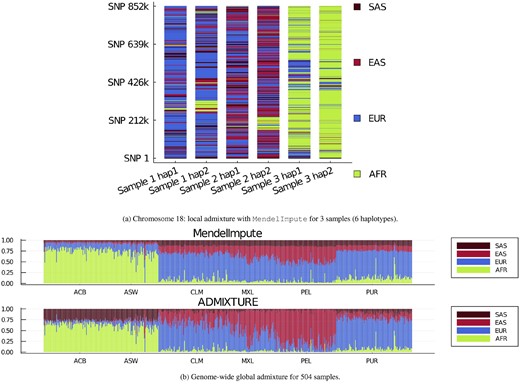
(a) Local ancestry inference on chromosome 18 using MendelImpute. Sample 1 is Puerto Rican (PUR), sample 2 is Peruvian (PEL) and sample 3 is African American (ASW). Other abbreviations are explained in the text. (b) All (n = 504) samples’ global ancestry proportions estimated using all chromosomes. Each column is a sample’s admixture proportion. Samples used in (a) are located at index 2, 339 and 500.

We compared MendelImpute to our ADMIXTURE (Alexander et al., 2009) software using K = 4 populations. Figure 3b displays every admixed sample’s (n = 504) global admixture proportions. Both programs qualitatively agree for samples from the CLM, MXL and PUR populations. However, ADMIXTURE assigned $\sim 25\%$ South Asian ancestry to the two populations with African ancestry (ACB, ASW) whereas MendelImpute predicts $\sim 20\%$ Europeans for them. Previous studies (Bryc et al., 2010; Lind et al., 2007) suggest African Americans have $\sim 20\%$ European ancestry, so MendelImpute delivered the more reliable estimate. On the other hand, ADMIXTURE finds $>70\%$ East Asian ancestry (proxy for Amerindians) in Peruvians (PEL), whereas MendelImpute predicts equal ancestry split between European and South/East Asians. Based on previous admixture studies (Norris et al., 2018, 2020), Peruvians tend to have 50–90% Amerindian ancestries, so ADMIXTURE appears more reliable in this case. It is noteworthy that the cited Peruvian studies both used the ADMIXTURE software to infer ancestry, while the African American studies did not. Nevertheless, the fact that MendelImpute sometimes performs better than ADMIXTURE suggests caution. The addition of proper Amerindian samples to the reference panels would likely clarify results and bring the two programs into closer agreement.

3.4 Ultra-compressed phased genotype files

As discussed earlier, VCF files are enormous and slow to read. If genotypes are phased with respect to a particular reference panel, then an alternative is to store each haplotype segment’s starting position and a pointer to its corresponding reference haplotype. This offers massive compression because long haplotype segments are reduced to two integers. Instead of outputting compressed VCF files, which is the default, MendelImpute can optionally output such ultra-compressed phased data. Table 4 shows that the ultra-compressed format gives 20–270-fold compression compared to standard compressed VCF output. In principle, all phased genotypes can be stored in such files. The drawback is that compressed data can only be decompressed with the help of the original reference panel. Thus, this tactic relies on universal storage and curation of reference haplotype panels. These panels should be stored on the cloud for easy access and constructed so that they can be consistently augmented by new reference haplotypes.

Table 4.

Output file size comparison of compressed VCF and ultra-compressed formats

Dataset	vcf.gz size (MB)	Ultra-compressed size (MB)	Compression ratio
Sim 10K	10.07	0.05	201
Sim 100K	10.71	0.04	267
Sim 1M	11.05	0.04	276
1000G Chr10	24.04	0.43	56
1000G Chr20	10.69	0.25	43
HRC Chr10	157.76	6.01	26
HRC Chr20	70.93	3.47	20

4 Discussion

We present MendelImpute, the first scalable, data-driven method for phasing and genotype imputation. MendelImpute and supporting OpenMendel software (Zhou et al., 2020) provide an end-to-end analysis pipeline in the Julia programming language that is typically 10–100 times faster than methods based on HMMs, including Impute 5, Beagle 5.1 (Java) and Minimac 4 (C++). The speed difference increases dramatically as we increase the number of typed SNPs. Thus, denser SNP chips potentially benefit more from MendelImpute’s design. Furthermore, MendelImpute occupies a smaller memory footprint. This makes it possible for users to run MendelImpute on standard desktop or laptop computers on very large datasets such as the HRC. Unfortunately, we cannot yet have the best of both worlds, as MendelImpute exhibits a 1.5–2.2-fold worse error rate on real data. However, as seen in Table 3, MendelImpute’s error rate is still acceptably low. One can improve its error rate by implementing strategies that detect recombinations within windows (Liu et al., 2013) or that phase by dynamic programming as discussed in the Supplementary Material. Regardless, it is clear that big data methods can compete with HMM based methods on the largest datasets currently available and that there is still room for improvement and innovation in genotype imputation.

Beyond imputation and phasing, our methods extend naturally to ancestry estimation and data compression. If each reference haplotype is labeled with its country or region of origin, then MendelImpute can decompose a sample’s genotypes into segments of different reference haplotypes colored by these origins. The cumulative lengths of these colored segments immediately yield an estimate of admixture proportions. These results are comparable and possibly superior to those provided by ADMIXTURE (Alexander et al., 2009). Countries can be aggregated into regions if too few reference haplotypes originate from a given country. The colored segments also present a chromosome barcode that helps one visualize subject variation, recombination hotspots and global patterns of linkage disequilibrium. Data compression is achieved by storing the starting positions of each segment and its underlying reference haplotype. This leads to output files that are 20–270-fold smaller than standard compressed VCF files. Decompression obviously requires ready access to stable reference panels stored on accessible sites such as the cloud. Although such an ideal resource is currently part dream and part reality, it could be achieved by a concerted international effort.

For potential users and developers, the primary disadvantage of MendelImpute is its reliance on the importation and storage of a haplotype reference panel. Acquiring these panels requires an application process which can take time to complete. Understanding, storing and wrangling a panel add to the burden. The imputation server for Minimac 4 thrives because it relieves users of these burdens (Das et al., 2016). Beagle 5.1 and Impute 5 are capable of fast parallel data import on raw VCF files (Browning et al., 2018) that neither Minimac 4 nor MendelImpute can currently match. This makes target data import, and especially preprocessing the reference panel, painfully slow for both programs. Fortunately, preprocessing only has to happen once.

Finally, let us reiterate the goals and achievements of this paper. First, we show that data-driven methods are competitive with HMM methods on genotype phasing and imputation, even on the largest datasets available today. Second, we challenge the notion that prephasing and imputation should be kept separate; MendelImpute performs both simultaneously. Third, we argue that data-driven methods are ultimately more flexible; for instance, MendelImpute readily handles imputation and phasing on dosage data. Fourth, we demonstrate that data-driven methods yield dividends in ancestry identification and data compression. Fifth, MendelImpute is completely open source, freely downloadable and implemented in Julia, an operating system agnostic, high-level programming language for scientific research. Julia is extremely fast and enables clear modular coding. Our experience suggests that data-driven methods will offer a better way forward as we face increasingly larger reference panels, denser SNP array chips and greater data variability.

Acknowledgements

We would like to thank Calvin Chi for his helpful discussions on ancestry estimation and Juhyun Kim for her helpful discussions on imputation quality scores.

Funding

B.C. and R.W. were supported by NIH grant T32-HG002536. B.C., E.S., J.S., H.Z. and K.L. were supported by NIH grant R01-HG006139. E.S., J.S., H.Z. and K.L. were supported by NIH grants R01-GM053275 and R35-GM141798. J.S. was also supported by NIH grant R01-HG009120. H.Z. was also supported by NSF grant DMS-2054253.

Conflict of Interest: none declared.

Data availability

All commands needed to reproduce the results we present are available at the MendelImpute site in the "manuscript" sub-folder. SnpArrays.jl is available at https://github.com/OpenMendel/SnpArrays.jl. VCFTools.jl is available at https://github.com/OpenMendel/VCFTools.jl. The Haplotype Reference Consortium data is available at https://www.ebi.ac.uk/ega/datasets/EGAD00001002729. Raw 1000 genomes data is available at ftp://ftp.1000genomes.ebi.ac.uk/vol1/ftp/release/20130502/, and Beagle’s webpage https://bochet.gcc.biostat.washington.edu/beagle/1000_Genomes_phase3_v5a provides a quality controlled 1000 genomes data which we used in our experiments.