minMLST: machine learning for optimization of bacterial strain typing

Abstract

Motivation

High-resolution microbial strain typing is essential for various clinical purposes, including disease outbreak investigation, tracking of microbial transmission events and epidemiological surveillance of bacterial infections. The widely used approach for multilocus sequence typing (MLST) that is based on the core genome, cgMLST, has the advantage of a high level of typeability and maximal discriminatory power. Yet, the transition from a seven loci-based scheme to cgMLST involves several challenges, that include the need by some users to maintain backward compatibility, growing difficulties in the day-to-day communication within the microbiology community with respect to nomenclature and ontology, issues with typeability, especially if a more stringent approach to loci presence is used, and computational requirements concerning laboratory data management and sharing with end-users. Hence, methods for optimizing cgMLST schemes through careful reduction of the number of loci are expected to be beneficial for practical needs in different settings.

Results

We present a new machine learning-based methodology, minMLST, for minimizing the number of genes in cgMLST schemes by identifying subsets of informative genes and analyzing the trade-off between gene reduction and typing performance. The results achieved with minMLST over eight bacterial species show that despite the reduction in the number of genes up to a factor of 10, the typing performance remains very high and significant with an Adjusted Rand Index that ranges between 0.4 and 0.93 in different species and a P-value < ${10}^{-3}$⁠. The identification of such optimized MLST schemes for bacterial strain typing is expected to improve the implementation of cgMLST by improving interlaboratory agreement and communication.

Availability and implementation

The python package minMLST is available at https://PyPi.org/project/minmlst/PyPI and supported on Linux and Windows.

Supplementary information

Supplementary data are available at Bioinformatics online.

1 Introduction

High-resolution microbial strain typing, or classifying bacteria at the strain level, is essential for various clinical purposes, including disease outbreak investigation, tracking of microbial transmission events and epidemiological surveillance of bacterial infections. In recent years, Whole Genome Sequencing (WGS) of bacteria has become increasingly available to microbiology laboratories and is recognized to be a new gold standard for typing.

Strain typing is primarily achieved by single-nucleotide polymorphism (SNP) or gene-by-gene comparisons (Schürch et al., 2018), where the latter approach provides the advantages of standardization, scalability, and ease of data sharing among laboratories. The most widely used gene-by-gene approach is based on multilocus sequence typing (MLST), comprised typing schemes that use a different number of loci (i.e. genes) each is suitable for addressing different levels of isolate discrimination (Maiden et al., 2013). Approaches based on smaller subsets of genes are the 7-locus conventional MLST (Li et al., 2009) and the 53-locus ribosomal MLST (rMLST) (Jolley et al., 2012). The conventional MLST can discriminate species and lineages but its discriminatory power is not sufficient for high-resolution typing (Maiden et al., 2013). It has also been shown that the 53 ribosomal genes are not necessarily superior to the 7 traditional genes in the identification of bacterial strains since these genes are very conserved (Alikhan et al., 2018; Pearce et al., 2018).

With the advent of WGS, MLST has been greatly enhanced and schemes for typing based on the bacterial core genome (cgMLST) or whole genome (wgMLST) are increasingly becoming available. A typical cgMLST scheme involves hundreds or more than a thousand loci, having a high level of typeability and maximal discriminatory power (Dekker et al., 2016; Maiden et al., 2013).

The MLST schemes have been defined and adopted for many microbial species, and thousands of MLST profiles and sequences, especially of pathogens, are available online in continuously updated public databases, such as (pubmlst.org), (mlst.net) and (cgMLST.org) (Dekker et al., 2016; Zolfo et al., 2017). Such databases provide portable nomenclature schemes and enable convenient data sharing within and across laboratories (Maiden et al., 2013; Schürch et al., 2018).

While cgMLST has notable advantages, the transition from a seven loci-based scheme to cgMLST involves several challenges. These challenges include (i) the need by some users to maintain backward compatibility, although this may prove difficult to maintain over time (ii) growing difficulties in the day-to-day communication within the microbiology community with respect to nomenclature and ontology, especially in the light of the increasing complexity of allelic profiles, (iii) issues with typeability, especially if a more stringent approach to loci presence is used (since an increasing number of loci increases the likelihood of typeability issues) and (iv) computational requirements concerning laboratory data management and sharing with end-users. Hence, methods for optimizing cgMLST schemes through careful reduction of the number of loci are expected to be beneficial for practical needs in different settings.

Several approaches have been suggested for identifying a reduced subset of genes that preserves high discrimination. Following the publication of the first cgMLST scheme for Legionella pneumophila (Moran-Gilad et al., 2015), David et al. extracted random nested subsets of 50, 100 and 500 genes from the core genes of the organism, and assessed the discriminatory power of these sets using the index of discrimination (D) previously suggested by Hunter et al. (1988). They found that a scheme of ∼50 genes offered the best compromise between improved discrimination (D = 0.99) and good epidemiological concordance (0.941). To identify potential discriminatory genes of Mycoplasma hominis, Jironkin et al. (2016) suggested a leave-one-out methodology according to which a gene is selected for the minimal MLST scheme in case its removal from the cgMLST scheme muddles the phylogenetic relationship of the isolates with respect to the whole genome SNP phylogenetic tree. Their minimal set included 48 genes required to recapitulate the phylogenetic relationships found using whole-genome SNPs.

In this article, we propose an efficient, generic and interpretable machine learning-based methodology, which we call minMLST. minMLST aims to minimize the number of genes in any given MLST scheme by quantifying gene importance and evaluating the strain typing performance on reduced subsets of informative genes. Our methodology was implemented into a publicly available software that can be easily installed from https://pypi.org/project/minmlst/PyPl. We applied minMLST on eight different bacterial schemes and achieved a reduction in the number of genes up to a factor of 10 while preserving high discrimination among strains with an Adjusted Rand Index (ARI) that ranges between 0.4 and 0.93 in different species with a P-value below ${10}^{-3}$⁠.

2 Materials and methods

minMLST is a hybrid methodology that combines both supervised and unsupervised machine learning algorithms, as outlined in Figure 1. We first provide a formal description of the algorithmic components, measures and statistical tests that are used in the methodology. Then the algorithms of minMLST are outlined and elaborated in detail.

Fig. 1.

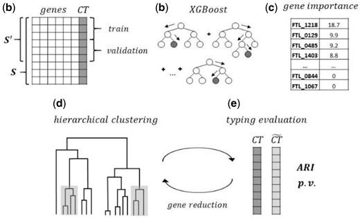
The workflow of minMLST methodology in high-level. (a) Filtering cluster-types ( ) with a single isolate (singletons) from the original cgMLST scheme; then splitting the isolates in the filtered scheme into train and validation sets. (b) Training an XGBoost classifier until a minimal Multiclass Log Loss is achieved on the validation set. (c) Quantifying gene importance in the trained XGBoost model using a selected measure (the mean magnitude of the SHAP values, weight, gain, or cover). Next, repeating steps (d) and (e) iteratively for a reduced number of most important genes: (d) Performing strain typing of all isolates in scheme using a distance-based hierarchical clustering; (e) Evaluating typing performance by applying a significance test to the Adjusted Rand Index ( ), comparing the types induced by minMLST ( ) and the ground-truth cluster-types predefined in the original cgMLST scheme

2.1 XGBoost

The main building block of our proposed methodology is the XGBoost algorithm that is used for identifying informative genes (i.e. features) in an input bacterial scheme. XGBoost is a regularized variant of Gradient Boosting Machines (GBM) (Chen et al., 2016), which has demonstrated superior performance in many machine learning competitions and studies in various fields (Babajide Mustapha et al., 2016; Fan et al., 2018; Georganos et al., 2018; Möller et al., 2016; Tamayo et al., 2016) including bioinformatics (Pang et al., 2019; Wang et al., 2019; Yu et al., 2019; Zou et al., 2018). Its objective function combines a loss function and additional regularization factor to control the complexity of the model and reduce overfitting. XGBoost is an ensemble of Classification and Regression Trees (CART), as each tree-classifier added to the ensemble constantly improves over previous classifiers’ error (Georganos et al., 2018).

2.2 Agglomerative hierarchical clustering

Agglomerative hierarchical clustering methods construct clusters by recursively merging similar objects in a bottom-up manner. The similarity between any pair of objects is usually quantified as a measure of distance, and a linkage method is used to determine the distance between any two clusters, as a function of the pairwise distances between their objects (Rokach et al., 2005). The result is a dendrogram that demonstrates the nested grouping of objects and the similarity levels measured at each grouping step. To obtain a specific partition, a threshold is applied for the required level of similarity.

2.3 Measures

The following measures are used in two parts of our methodology: SHAP values and measures specific for tree-based models are used for gene importance quantification, whereas the ARI and its significance P-value are used for the evaluation of strain typing performance. Pearson’s and Spearman’s correlations are used for comparing the gene importance values computed with different measures.

2.3.1 SHAP values

The SHapley Additive exPlanations (SHAP) values suggested by Lundberg and Lee constitute a unified measure of feature importance, which enables to interpret the predictions of complex models, such as tree ensembles or deep neural networks (Lundberg et al., 2017). The SHAP values attribute to each feature the change in the expected model prediction when conditioning on that feature. Unlike other feature attribution methods that are inconsistent and may lower the feature’s assigned importance when the true impact of that feature actually increases, the SHAP values are theoretically optimal, being the unique consistent and locally accurate feature attribution values (Lundberg et al., 2018). The SHAP values enable local interpretability since they measure the contribution of each feature to the prediction of a specific sample, therefore different (local) explanations can be provided for different samples. Computing the SHAP values may be challenging, yet for tree-ensembles, the complexity of computation can be reduced exponentially using a dedicated algorithm, e.g. TreeSHAP (Lundberg et al., 2018). In our methodology, we use the mean absolute value of the SHAP values, a.k.a. the mean magnitude of the SHAP values, of each feature (i.e. gene) to quantify its average impact on the model output magnitude.

2.3.2 Measures specific for tree-based models

We use additional measures that are specific to tree-based models (including XGBoost) for quantifying feature importance: weight, cover and gain. Weight (a.k.a. split-count) is the number of times a given feature is used to split the data across all splits. The average (or total) cover is the average (or total) quantity of samples conditioned on a given feature across all splits. Average (or total) gain is the average (or total) reduction in the Multiclass Log Loss (i.e. the objective function) contributed by a given feature across all splits. Given a dataset of $N$ samples and $K$ labels; Let $Y$ be a binary indicator matrix that encodes true labels and $P$ be a matrix of probability estimates, the Multiclass Log Loss is defined as:

$$L_{\log }\left(Y,\mathrm{ }P\right)=\mathrm{ }-\frac{1}{N}\sum _{i=0}^{N-1}\sum _{k=0}^{K-1}{y}_{i,k}\log p_{i,k},$$

(1)

 

$$\mathrm{where}\mathrm{ }{y}_{i,k}=\mathrm{ }\left\{\begin{array}{c}1 if \mathit{sample} i \mathit{has} \mathit{label} k\\ 0 \mathit{else}\end{array}\right.$$

 

$${\mathrm{ }p}_{i,k}=\mathrm{Pr}\left(y_{i,k}=1\right).$$

2.3.3 Pearson’s and Spearman’s correlations

To compare gene importance values computed by different measures, we use Pearson’s correlation which assesses the linear relationship between two continuous variables and Spearman’s rank-order correlation which assesses the monotonic relationship between two continuous or ordinal variables.

2.3.4 Adjusted Rand Index

The ARI is a known evaluation criterion, which measures the similarity between two different partitions of a set of objects. It is based on pair-wise comparisons of objects assignment to clusters (i.e. are the two objects in the same cluster or not), in addition to being corrected for chance (Hubert et al., 1985). Formally, given a dataset of $n$ objects, suppose $U=\{u_1, \dots ,u_i,\dots ,u_r\}$and $V=\{v_1, \dots ,v_j,\dots ,v_c\}$represent two different partitions of the objects set, the $\mathit{ARI}$ between $U$ and $V$ is defined as:

$${\mathrm{ARI}}_0=\mathrm{ }\frac{\sum _{i,\mathrm{ }j}\left(\begin{array}{c}{n}_{i,j}\\ 2\end{array}\right)-\sum _i\left(\begin{array}{c}{n}_{i·}\\ 2\end{array}\right)\sum _j\frac{\left(\begin{array}{c}{n}_{·j}\\ 2\end{array}\right)}{\left(\begin{array}{c}n\\ 2\end{array}\right)}}{\frac{1}{2}\mathrm{ }\left[\sum _i\left(\begin{array}{c}{n}_{i·}\\ 2\end{array}\right)+\sum _j\left(\begin{array}{c}{n}_{·j}\\ 2\end{array}\right)\right]-\sum _i\left(\begin{array}{c}{n}_{i·}\\ 2\end{array}\right)\sum _j\frac{\left(\begin{array}{c}{n}_{·j}\\ 2\end{array}\right)}{\left(\begin{array}{c}n\\ 2\end{array}\right)}},$$

(2)

where n_i is the number of objects in cluster u_i, n_·j is the number of objects in cluster v_j, n_ij is the number of objects that are common to clusters u_i and v_j.

To assess the significance of the observed $\mathit{ARI}$ (⁠${\mathit{ARI}}_0$⁠) Qannari et al. suggested a permutation test based on a Monte Carlo simulation (Qannari et al., 2014). It involves the simulation of ∼1000 pairs of partitions for estimating the distribution of the $\mathit{ARI}$ test statistic, under the null hypothesis stipulating the absence of association between the two partitions being compared (Qannari et al., 2014). This significance test provides a good estimation but may be time consuming.

2.4 Threshold definition

In our methodology, we use agglomerative hierarchical clustering where the distance between any pair of isolates is defined as the proportion of genes that disagree on their allelic assignment, and the distance between any two clusters is determined by a linkage method. To obtain the partition into clusters, we apply a threshold on the distance between isolates belonging to the same cluster type. As the distance between any pair of isolates is computed based on a given subset of genes, we do not have any prior knowledge about the distribution of the pairwise distances. This distribution may also change when different subsets of genes are selected, e.g. the distances’ distribution of Enterococcus faecium when selecting all its 1423 genes versus a subset of 88 genes (see Supplementary Table S1). Thus, we use percentile-based thresholds instead of constant thresholds. For a given percentile, we dynamically calculate the threshold value for each subset of genes.

2.5 Proposed methodology

The first step of our proposed minMLST methodology (Algorithm 1) is the training of an XGBoost classifier. This is a supervised learning process that requires ground-truth labels as input, which are, in our case, the cluster types (CTs). To split the data into training and validation sets so that each type will be represented in both sets, we first filtered out CTs with a single isolate (i.e. singletons) (Lines 1–2). The exclusion of the singletons also removes some potential noise from the training process, letting the XGBoost model focus on more prevalent cluster types, under the assumption that the informative genes found by this process will be able to generalize the entire dataset when performing the strain typing (Algorithm 2). The XGBoost is trained for minimizing the Multiclass Log Loss metric. To control overfitting, we track the performance of the model at each training epoch and stop the training process when a minimal Multiclass Log Loss is achieved on the validation set (Line 3). The second step of the methodology is to quantify the importance level of each gene in the trained model using one of the following measures: the mean magnitude of the SHAP values, weight, average gain, total gain, average cover, or total cover (Line 4). For each of the above measures, a high value reflects a high importance level. Next, we iteratively examine various percentiles to be used for calculating the thresholds in the clustering algorithm (Lines 5–12).

Algorithm 1 Pseudocode of the minMLST methodology

$\mathit{Inputs}$⁠:

• $S$ – a bacterial scheme in a matrix format with m rows and n columns: the n-1 columns correspond to genes, the last column n contains the ground-truth cluster-type (CT). Each row m represents an allelic profile of a single isolate.

• $\mathit{measure}$ – the measure according to which the importance level of each gene is calculated. Can be either the mean magnitude of the SHAP values, weight, average gain, total gain, average cover, or total cover.

• $r$ – the number of genes to be removed at each iteration.

• $\mathit{linkage}$ – the linkage method to compute the distance between clusters. Can be either single, complete, average, weighted, centroid, median, or ward.

• $P$ – a list of percentiles to be evaluated, sorted in ascending order.

  1. Filter cluster-types with a single isolate (singletons) from $S$⁠, resulting in a filtered scheme $S\prime$⁠.

  2. Split isolates in $S\prime$ into train and validation sets in a stratified manner, so that each cluster-type has at least one isolate in each set.

  3. Train an XGBoost classifier until a minimal Multiclass Log Loss is achieved on the validation set.

  4. Quantify gene importance $GI$ in the trained model according to $\mathit{measure}$⁠.

  5. $\overrightarrow{AR{I}_{\mathit{best}}}$⁠, $\overrightarrow{{p.v}_{\mathit{best}}}$ = Algorithm 2 ($\mathit{S},\mathit{r},\mathit{linkage},{\mathit{GI},\mathit{P}}_0$)

  6. For $i$ in $\mathit{range}(1, \mathit{len}\left(P\right))$⁠:

  7. $\overrightarrow{AR{I}_{\mathit{next}}}$⁠, $\overrightarrow{{p.v}_{\mathit{next}}}$ = Algorithm 2 ($\mathit{S},\mathit{r},\mathit{linkage},{\mathit{GI},\mathit{P}}_{\mathit{i}}$)

  8. $d=\sum _k({\overrightarrow{AR{I}_{\mathit{next}}}}_k-{\overrightarrow{AR{I}_{\mathit{best}}}}_k)$

  9. if $d$  $\ge$ 0:

  10. $\overrightarrow{AR{I}_{\mathit{best}}}$⁠, $\overrightarrow{{p.v}_{\mathit{best}}}$ = $\overrightarrow{AR{I}_{\mathit{next}}}$⁠, $\overrightarrow{{p.v}_{\mathit{next}}}$

  11. else:

  12. $\mathit{break}$

$\mathit{Outputs}$⁠:

• $GI$ – importance score per gene according to $\mathit{measure}$⁠.

• $\overrightarrow{AR{I}_{\mathit{best}}}$ , $\overrightarrow{{p.v}_{\mathit{best}}}$ – a vector of the Adjusted Rand Index (respectively P-value) computed for each subset of most important genes, when using the best percentile in $P.$

Algorithm 2 Pseudocode of typing performance evaluation for a given percentile

$\mathit{Inputs}$⁠:

• $S,\mathrm{ }r,\mathrm{ }\mathit{linkage}$ – see Algorithm 1.

• $GI$ – importance score per gene.

• $p$ – a percentile to be examined.

1. ${\mathit{subset}}_{\mathit{complete}}$= all genes in $GI$⁠.

2. ${\mathit{subset}}_{\mathit{imp}}$ = all genes in $GI$ with importance score > 0.

3. ${\mathit{subset}}_{\mathit{imp}-i\mathrm{*}r}$ = the remaining genes after removing the $i\mathrm{*}r$ least important genes from ${\mathit{subset}}_{\mathit{imp}}$  $i=\left(1,\mathrm{ }2,\mathrm{ }\dots ,\mathrm{ }n\right),\mathrm{ }\mathit{where}\mathrm{ }n<\frac{\mathit{len}\left({\mathit{subset}}_{\mathit{imp}}\right)}{r}.$

4. $\mathit{subsets}$ = [${\mathit{subset}}_{\mathit{complete}},\mathrm{ }{\mathit{subset}}_{\mathit{imp}},\mathrm{ }{\mathit{subset}}_{\mathit{imp}-i\mathrm{*}r}\mathrm{ },\mathrm{ }\dots \mathrm{ },$  ${\mathit{subset}}_{\mathit{imp}-n\mathrm{*}r}$]

5. $\overrightarrow{\mathit{ARI}}\mathrm{ }$⁠, $\overrightarrow{p.v}$ = [ ], [ ]

6. For each $\mathit{subset}$ in $\mathit{subsets}$⁠:

7.  Minimize the input scheme $S$ to include only the $\mathit{subset}$ of genes.

8.  Compute a normalized Hamming distance between each pair of isolates in $S$⁠.

9.  Construct agglomerative hierarchical clustering based on the distances matrix between all isolates, using the $\mathit{linkage}$ method.

10.  Compute distances’ distribution.

11.  Set $\mathit{threshold}\mathrm{ }$= percentile $p$ of distances’ distribution.

12.  Apply the $\mathit{threshold}$ to get an induced cluster-type per isolate (i.e. induced partition).

13.  Compute the Adjusted Rand Index (⁠$\mathit{ARI}$⁠) between the induced cluster-types and the ground-truth cluster-types (provided in the last column of $S$⁠).

14.  Compute the P-value of the $\mathit{ARI}$ using a permutation test.

15.  Append $\mathit{ARI}$ and P-value to $\overrightarrow{\mathit{ARI}}\mathrm{ }$⁠, $\overrightarrow{p.v}$ respectively.

$\mathit{Ouput}$⁠:

• $\overrightarrow{\mathit{ARI}}\mathrm{ }$⁠, $\overrightarrow{p.v}$ – Adjusted Rand Index (corresponding P-value) computed for each subset of genes when using a given percentile.

The evaluation of the typing performance when using a certain percentile is depicted in Algorithm 2. We analyze how a machine learning-guided reduction in the least important genes affects the typing performance, starting from the complete input scheme that includes all genes (Line 1), continuing with a scheme that includes only informative genes (Line 2) and then iteratively reducing the $r$ least important genes from the previous scheme (Line 3). Each subset of genes is evaluated as follows: First, we compute the normalized Hamming distance between every pair of isolates (their allelic profiles) to quantify the proportion of the genes which disagree on their allelic assignment. These pairwise distances between all isolates are stored in a matrix (Line 8). Second, we perform agglomerative hierarchical clustering based on the distances matrix, while the distance between any two clusters is determined according to a selected linkage method, e.g. single, complete, average, weighted, centroid, median or ward (Rokach et al., 2005) (Line 9). We compute the distribution of the pairwise distances and use the $p$ percentile as a threshold for clustering (Lines 10-11). Third, we evaluate the typing performance by comparing the induced types and the ground-truth cluster types predefined by the original cgMLST scheme, using the ARI (Line 12). Fourth, we compute the P-value of the observed $\mathit{ARI}$ by implementing a permutation test suggested by Qannari et al. (2014) (Line 13). The outputs of Algorithm 2 are the $\mathit{ARI}$ and P-value results computed for each subset of genes, when using a given percentile.

The $\mathit{ARI}$ results computed by Algorithm 2 are then used in Algorithm 1 for the process of finding a recommended percentile. This is the percentile with the best overall predictive performance, which is equivalent to the $\mathit{ARI}$ curve with the highest AUC, and is referred to as ‘best’. At first, we initialize ‘best’ to the minimal percentile in search space $P$ (Line 5). Then we compare ‘best’ to the successor percentile in $P$⁠, referred to as ‘next’, by computing the ‘non-absolute’ L1 distance between their $\mathit{ARI}$ vectors. This distance equals to the sum of the differences between the two vectors when subtracting the ‘best’ from the ‘next’ (Lines 6–8). In case the distance is not negative (i.e. ‘next’ performs better or the same), ‘next’ is defined as the new ‘best’ (Lines 9–10). Otherwise, the search is completed and ‘best’ is selected as the recommended percentile (Lines 11-12). The outputs of Algorithm 1 are the gene importance scores according to the input $\mathit{measure}$⁠, and the $\mathit{ARI}$ and P-value results computed for each subset of genes when using the best percentile in $P.$

2.5.1 Implementation

The minMLST tool is implemented in Python 3 and is applicable for both Windows and Linux platforms. It supports parallel computing and can be easily installed from https://pypi.org/project/minmlst/PyPI. Detailed documentation and usage examples are available on https://github.com/shanicohen33/minMLSTGitHub.

3 Results

3.1 Datasets

Data were retrieved on June 2018 from the cgMLST.org server which hosts the allelic nomenclature of core genome MLST (cgMLST) gene schemes, generated by the (Ridom SeqSphere+) commercial software. We used the allelic profiles of thousands of isolates belonging to eight different pathogenic species that are responsible for a significant global bacterial disease burden. The characteristics of the cgMLST scheme of each bacterial species are detailed in Table 1.

Table 1.

Characteristics of cgMLST schemes of selected pathogens

Scheme	No. of loci	No. of isolates indexed	Cluster type count	Cluster type distance	Distance/no. of genes	References
F.tularensis	1147	240	145	1	0.087	Antwerpen et al. (2015)
L.pneumophila	1521	811	356	4	0.263	Moran-Gilad et al. (2015)
C.difficile	2270	4450	2425	6	0.264	Bletz et al. (2018)
A.baumannii	2390	4594	1936	9	0.377	Higgins et al. (2017)
K.pneumoniae	2358	5833	2174	15	0.636	Weber et al. (2019) and Piazza et al. (2019)
E.faecium	1423	10 550	1833	20	1.405	de Been et al. (2015)
L.monocytogenes	1701	17 566	6426	10	0.588	Ruppitsch et al. (2015)
S.aureus	1861	20 136	9868	24	1.29	Leopold et al. (2014)

Scheme = bacterial species; No. of loci = number of core genes included in the scheme; No. of isolates indexed = number of isolates (allelic profiles) deposited in the database; Cluster type count = number of different types (different allelic profiles) assigned to deposited isolates; Cluster type distance = threshold for the maximal number of different alleles between isolates of the same cluster type, as described in the original publication of each scheme; Distance/No. of genes = cluster type distance divided by the number of core genes.

3.2 XGBoost training and validation

We trained an XGBoost model for each bacterial species, tracking both the Multiclass Log Loss and the Multiclass error over the train and the validation sets. For most bacterial datasets, 100 training epochs were sufficient to reach a minimal Multiclass Log Loss over the validation set, with the exception of Staphylococcus aureus and E.faecium that reached a plateau after 170 and 400 epochs, respectively. For space considerations, Figure 2 and all the following figures present the results for L.pneumophila and E.faecium. The results for the remaining six bacterial species are provided in Supplementary Materials (see Supplementary Fig. S1 for XGBoost performance evaluation).

Fig. 2.

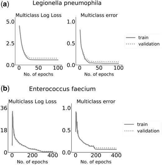
Metrics of the XGBoost model along the training process. Multiclass Log Loss (objective function) and multiclass error values on the train and validation sets are presented as a function of the training epochs for (a) L.pneumophila and (b) E.faecium

3.3 Quantification of gene importance

Gene importance was quantified with six different measures (described in Section 2.2): the mean magnitude of the SHAP values, weight, average gain, average cover, total gain and total cover. We then compared the gene importance values for each pair of measures. We found a high Pearson’s (⁠$P$⁠) and Spearman’s (⁠$S$⁠) correlations between the SHAP and total gain importance values computed for L.pneumophila (⁠$P$=0.85, $S$=0.88) and E.faecium (⁠$P$=0.77, $S$=0.87), as presented in Figure 3. Similar results were also found for Francisella tularensis (⁠$P$=0.96, $S$=0.88), Clostridioides difficile (⁠$P$=0.55, $S$=0.89), Acinetobacter baumannii (⁠$P$=0.72, $S$=0.86), Klebsiella pneumoniae (⁠$P$=0.84, $S$=0.88), Listeria monocytogenes (⁠$P$=0.9, $S$=0.79) and S.aureus (⁠$P$=0.24, $S$=0.83), as presented in Supplementary Figure S2. In all bacteria, relatively high Spearman’s correlations (⁠$S$≥0.64) were observed between the SHAP, total cover, total gain and weight importance values, as presented in Figure 3 and Supplementary Figure S2. Gene importance values for all bacteria are provided in Supplementary File S1.

Fig. 3.

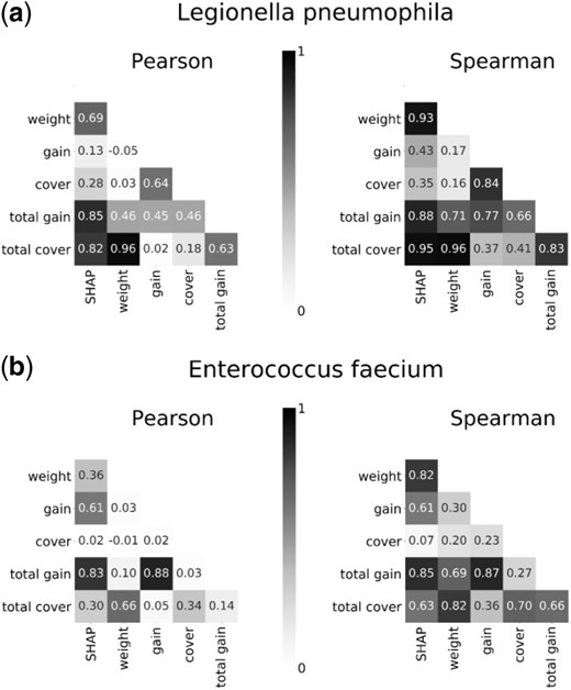
Pearson’s and Spearman’s correlations between gene importance values computed by six different measures for (a) L.pneumophila and (b) E.faecium. The measures that were used for gene importance quantification are the mean magnitude of the SHAP values, weight, average gain, average cover, total gain and total cover

3.4 Analyzing the trade-off between gene reduction and strain typing performance

We applied the minMLST methodology on the eight bacterial datasets to analyze the trade-off between learning-based gene reduction and strain typing performance. Gene importance was calculated based on the mean magnitude of the SHAP values as these values are consistent and locally accurate (Lundberg et al., 2017). The number of informative genes (importance score > 0) found for each bacteria was 133 (11.5%) for F.tularensis, 1030 (67.7%) for L.pneumophila, 2169 (95.5%) for C.difficile, 2347 (98.2%) for A.baumannii, 2100 (89%) for K.pneumoniae, 1088 (76.4%) for E.faecium, 1692 (99.4%) for L.monocytogenes and 1860 (99.9%) for S.aureus. We removed the least informative genes from each scheme in intervals of 100 genes, except for F.tularensis where intervals of 40 genes were used due to a low number of informative genes. For all bacteria, the distance between clusters was computed with the complete linkage method, and P-value calculations were based on 1000 simulated samples. For each bacterial species, we show the results obtained in the last three iterations of Algorithm 1, i.e. the results obtained with the best percentile and its two adjacent percentiles (predecessor and successor) in the search space of the algorithm (Fig. 4 and Supplementary Fig. S3). The search space included the following percentiles of distances’ distribution: [0.005, 0.01, 0.05, 0.1, 0.5, 1, 1.5, 2, …, 10]. For each iteration, we present the $\mathit{ARI}$ and P-value results computed for every subset of genes. In most bacteria, except for E.faecium, the best percentile was either the 0.5th or the 1st percentile of distances’ distribution. As for E.faecium, the algorithm found the 9th percentile as the best. This exception can be explained by the relatively high ratio of Distance/No. of genes that equals to 1.405 in the scheme of E.faecium (Table 1). This high ratio indicates that a higher percentage of different alleles was allowed between isolates belonging to the same cluster type of this bacterial species. Hence, it is reasonable that the best percentile found for this bacterium was higher, resulting in relatively higher thresholds for the distance between isolates of the same cluster type. To enable comparison with other bacteria, the results presented for E.faecium include also the 1st percentile of distances’ distribution (Fig. 4). The actual values of the thresholds are presented in Supplementary Table S1 per bacterial species and for each subset of genes.

Fig. 4.

ARI and P-value computed for each subset of most informative genes for (a) L.pneumophila and (b) E.faecium. We present the results obtained when using the complete linkage method with the best percentile and its two adjacent percentiles (predecessor and successor) in the search space of Algorithm 1. The search space included the following percentiles of distances’ distribution: [0.005, 0.01, 0.05, 0.1, 0.5, 1, 1.5, 2, …, 10]. For E.faecium, we also present the results with the 1st percentile of distances’ distribution, for comparison with the other bacteria

Figure 4 shows that despite the reduction in the number of genes up to a factor of 10, the $\mathit{ARI}$ remains very high and stable, ∼0.8 for L.pneumophila and between 0.8 and 0.93 for E.faecium. Also in the remaining bacterial species, the $\mathit{ARI}$ results are high, significant and decline very moderately with a tenfold reduction in the number of genes. The specific $\mathit{ARI}$ results are ∼0.5 for F.tularensis, 0.4–0.5 for C.difficile, ∼0.6 for A.baumannii, 0.5–0.6 for K.pneumoniae, 0.7–0.8 for L.monocytogenes and 0.5–0.6 for S.aureus (Supplementary Fig. S3). In all bacteria, the $\mathit{ARI}$ results were very significant with a P-value < ${10}^{-3}$⁠.

3.5 Visualization of strain typing results using phylogenetic trees

We next reconstructed phylogenetic trees based on the cgMLST allelic profiles of the bacterial isolates using a minimum spanning tree algorithm, MSTree V2, implemented in the GrapeTree tool (Zhou et al., 2018). We used the iTOL online tool (Letunic et al., 2007) to generate a visualization of the phylogenetic trees alongside a partition into cluster types, so that each cluster type is represented by a different color. This view provides a visual comparison between the cluster types induced by minMLST based on a minimal subset of genes and the ground-truth cluster types predefined by Ridom SeqSphere+ based on all core genes. The specific logic we developed for setting the colors is outlined in Supplementary Algorithm S1.

We present the phylogenetic trees of L.pneumophila and E.faecium in Figure 5. The inner colors’ ring (as well as the colors of the leaves) represents the predefined partition into cluster types provided by Ridom SeqSphere+ and the outer colors’ ring represents the partition induced by minMLST: 230 (15.1%) and 188 (13.2%) most informative genes obtained with the 0.5th percentile and 9th percentile for L.pneumophila and E.faecium, respectively. The visual comparison of typing results for the remainder bacteria is presented in Supplementary Figure S5, and is based on 133 (11.5%), 1569 (69.1%), 1547 (64.7%) and 700 (29.6%) most informative genes obtained with the 1st, 1st, 0.5th and 1st percentile for F.tularensis, C.difficile, A.baumannii and K.pneumoniae, respectively. Due to a memory limitation of the GrapeTree tool, we could not use the MSTree V2 algorithm for reconstructing the polygenetic trees of L.monocytogenes and S.aureus.

Fig. 5.

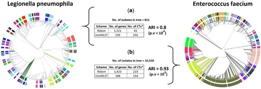
Phylogenetic trees of (a) L.pneumophila and (b) E.faecium reconstructed by the GrapeTree tool using the full cgMLST scheme. The inner colors’ ring represents the CTs predefined by Ridom SeqSphere+ based on all core genes, the outer colors’ ring represents the CTs induced by minMLST based on a minimal subset of informative genes. To keep a clear view, only CTs with more than five related isolates are colored in the inner ring, whereas the outer ring shows the corresponding typing results of these isolates according to minMLST (logic for color settings is depicted in Supplementary Algorithm S1). *No. of CTs—in Ridom’s scheme, it refers to the number of CTs with more than five related isolates, i.e. the number of CTs presented in the inner colors’ ring. In minMLST’s scheme, it refers to the number of CTs defined for these isolates according to minMLST, i.e. the number of CTs presented in the outer colors’ ring. The $\mathit{ARI}$ and P-value were calculated based on the typing results of all isolates

4 Discussion

Using optimized MLST schemes for bacterial strain typing is expected to improve the implementation of cgMLST by improving interlaboratory agreement and communication. In this article, we introduced a new hybrid methodology, minMLST, for minimizing the number of genes in cgMLST schemes by identifying subsets of informative genes and analyzing the trade-off between gene reduction and typing performance, allowing users to choose the preferable balance point. The visual comparison of the strain typing results illustrated the ability to discriminate among strains when using a compact set of informative genes found by minMLST. We also provided a generic implementation of our methodology, the minMLST tool, which supports the continuous growth in the number of isolates, as well as new CTs that are submitted to online databases.

Compared to previous studies in which the contribution of each gene to discrimination between strains was evaluated separately regardless of other genes (Jironkin et al., 2016), minMLST takes advantage of a tree-based ensemble which considers the marginal addition of information provided by a certain gene given various compositions of other genes. Moreover, in our experiments, genes were selected for reduced schemes based on the SHAP values that are consistent and theoretically optimal feature attribution values (Lundberg et al., 2018). This might be advantageous compared to random gene selection aimed at generating lean schemes (David et al., 2016). In our methodology, strain typing performance is measured by the ARI that compares the partition into cluster types induced by a minimal subset of genes versus a predefined partition that is based on a complete set of genes. The Index of discrimination previously used by (David et al., 2016) was not suitable for this work as it gives higher values to partitions with lower variance in the number of isolates belong to each cluster type, whereas minMLST strives to preserve the typing results achieved based on the full set of genes, even when this partition demonstrates an uneven distribution of isolates into cluster types.

The clustering of strains into types is an unsupervised problem by definition. The methodology, we proposed is not aimed for predicting CTs for new and unseen isolates, but rather optimizing the core genome MLST (cgMLST) scheme for isolates that already exist in the database, by minimizing the number of genes in the scheme. The evaluation of the typing performance is done by comparing the results of an unsupervised clustering algorithm when using different subsets of genes, whereas a supervised XGBoost algorithm is used only for the purpose of identifying informative genes in the given scheme. To avoid overfitting, the training and validation process (i.e. hyperparameter setting) of the XGBoost model is done over a filtered dataset that excludes all singletons (see singletons percentage in Table 2), which results in a model that is more general and less prone to explain idiosyncrasies in the data. The validation set enables us to stop the training process of the XGBoost at the transition point from the generalization stage to the memorization stage and hence limit the selection of non-cost-effective genes, i.e. genes that are non-informative for the clustering of most isolates. In Supplementary Figure S6, we demonstrate how the exclusion of singletons during the training and validation process affects the resulting schemes of different bacteria. For each subset of most informative genes, we compare the $\mathit{ARI}$ achieved when the XGBoost model was trained without singletons versus trained with half of the singletons selected randomly. For all bacteria, the results show either similar $\mathit{ARI}$ values for the two models or an advantage (a higher $\mathit{ARI}$ on average) to the model trained without singletons. In addition, we present how the reduction in the number of informative genes affects the number of singleton CTs in the resulting scheme generated by minMLST for each bacteria (see Supplementary Fig. S7). It can be seen that for most bacteria, the reduction in the number of informative genes leads to a moderate decrease in the number of singleton CTs in the resulting scheme.

Table 2.

Percentage of singleton clusters (CTs with a single related isolate)

Scheme	Singleton CTs (%)
F.tularensis	75.9
L.pneumophila	60.4
C.difficile	74.4
A.baumannii	52.6
K.pneumoniae	65.9
E.faecium	61.5
L.monocytogenes	64.8
S.aureus	70.4

In our study, we had to deal with two data-related challenges. The first challenge is related to clone-types’ assignment in the (Ridom SeqSphere+) system. This assignment is influenced by the order of submission of the original allelic profiles as well as by missing genotyping data, as described in detail in Supplementary Materials. As a result, we did not achieve $\mathit{ARI}$=1 when comparing Ridom’s predefined CTs to the minMLST CTs induced based on all genes, as one would expect. To overcome this issue, we generated new ground-truth CTs by applying hierarchical clustering over the complete cgMLST scheme with the thresholds defined in the original publication of each bacterial scheme (Table 1). These thresholds are controversial as they were defined arbitrarily by each study, and hence were used only for validation of the $\mathit{ARI}$⁠. The comparison of the minMLST CTs induced based on all genes with the new ground-truth CTs resulted in $\mathit{ARI}$=1 in all bacterial datasets. The second challenge we faced was a significantly high number of singleton clusters, i.e. CTs with a single related isolate (Table 2), as well as a high number of 2, 3 and 4 size clusters (see Supplementary Table S3). Such data structure limits the application and evaluation of ‘pure’ supervised machine learning methods for CT assignment (e.g. k-fold cross-validation of a multiclass classifier). These unique characteristics of the MLST data motivated us to develop a hybrid methodology, minMLST, which combines a ‘supervised’ approach for identifying informative genes along with an ‘unsupervised’ approach for CT assignment and typing evaluation.

In conclusion, this study showed that the minMLST methodology successfully identifies reduced subsets of genes, up to a factor of 10 from the complete set, that perverse a high discrimination among strains, as demonstrated for eight different bacterial species. Our tool enables to analyze the trade-off between reducing the number of genes in the cgMLST scheme versus preserving a high resolution between different strains, so one can select the desired balance point. Our methodology will contribute to the generation of optimized and potentially more compact bacterial cgMLST schemes consisting of the most informative genes, which is expected to improve the uptake and usability of cgMLST even further as well as to improve communications and data sharing across the microbiology community without hampering the resolution and discriminatory power of genomic typing for public health.

Acknowledgements

The authors thank Dr. João André Carriço for useful discussions and suggestions.

Funding

S.C. was supported by the Israeli Ministry of Science and Technology (fellowship No. 3-14385).

Conflict of Interest: none declared.