


Abstract
Intrinsically disordered protein regions interact with proteins, nucleic acids and lipids. Regions that bind lipids are implicated in a wide spectrum of cellular functions and several human diseases. Motivated by the growing amount of experimental data for these interactions and lack of tools that can predict them from the protein sequence, we develop DisoLipPred, the first predictor of the disordered lipid-binding residues (DLBRs).
DisoLipPred relies on a deep bidirectional recurrent network that implements three innovative features: transfer learning, bypass module that sidesteps predictions for putative structured residues, and expanded inputs that cover physiochemical properties associated with the protein–lipid interactions. Ablation analysis shows that these features drive predictive quality of DisoLipPred. Tests on an independent test dataset and the yeast proteome reveal that DisoLipPred generates accurate results and that none of the related existing tools can be used to indirectly identify DLBR. We also show that DisoLipPred’s predictions complement the results generated by predictors of the transmembrane regions. Altogether, we conclude that DisoLipPred provides high-quality predictions of DLBRs that complement the currently available methods.
DisoLipPred’s webserver is available at http://biomine.cs.vcu.edu/servers/DisoLipPred/.
Supplementary data are available at Bioinformatics online.
1 Introduction
Many proteins include one or more intrinsically disordered regions (IDRs), which are defined as segments of protein sequence that lack stable three-dimensional structure under physiological conditions (Dunker et al., 2001; Habchi et al., 2014; Oldfield et al., 2019a). Recent studies suggest that proteins with IDRs are common across all domains of life (Peng et al., 2015; Xue et al., 2012) and carry out many cellular functions (Dunker et al., 2002; Dyson and Wright, 2005). In particular, IDRs were shown to interact with proteins, DNA, RNA, lipids and a variety of small molecules (Balcerak et al., 2019; Fuxreiter et al., 2014; Hatos et al., 2020; Kjaergaard and Kragelund, 2017; Meng et al., 2015; Patil et al., 2010; Varadi et al., 2015,b; Wang et al., 2016a). However, only several hundred of these interactions were annotated experimentally (Hatos et al., 2020; Katuwawala et al., 2019a,b). This annotation gap has motivated the development of computational methods that use protein sequences to predict IDRs interacting with specific partner types (Ghadermarzi et al., 2020; Katuwawala et al., 2019a,b; Meng et al., 2017; Varadi et al., 2015a). Importance of these methods was underscored in the recent large community-driven Critical Assessment of protein Intrinsic Disorder (CAID) (Necci et al., 2021). CAID introduced a new category of disorder predictions that focus specifically on disordered binding regions, which attracted submissions from 11 methods. Moreover, recently released centralized webserver for the disorder prediction, DEPICTER, includes predictions of the interacting IDRs (Barik et al., 2020).
While IDRs interact with a wide range of partners, such as proteins, nucleic acids and lipids, nearly all current predictors focus on the protein-binding IDRs (Katuwawala et al., 2019a,b; Meng et al., 2017; Varadi et al., 2015a). A recent survey has identified 21 predictors of the IDRs that interact with proteins (Katuwawala et al., 2019,b). Some of more popular methods in this category include ANCHOR (Dosztanyi et al., 2009; Mészáros et al., 2018), MoRFpred (Disfani et al., 2012; Oldfield et al., 2019,b), MoRFChiBi (Malhis et al., 2016; Malhis and Gsponer, 2015) and OPAL (Sharma et al., 2018, 2019). In contrast, there is only one method, DisoRDPbind (Peng et al., 2017; Peng and Kurgan, 2015), for the prediction of the DNA and RNA interacting IDRs and no methods to address interactions with lipids. The lack of tools could be explained by the insufficient amount of the experimental data that was needed to train and assess the predictive models. However, recent releases of DisProt database have delivered large amounts of new experimental annotations (Hatos et al., 2020; Piovesan et al., 2017). More specifically, version 8.0 of Disprot (Hatos et al., 2020) provides about 50% more experimental annotations of the lipid binding IDRs when compared with the previous version 7.2 (Piovesan et al., 2017).
Lipids are implicated in many cellular functions including energy storage, signaling, regulation, insulating and transport (Dall'Armi et al., 2013; Di Paolo and De Camilli, 2006; Settembre et al., 2013; Soto-Avellaneda and Morrison, 2020; Welte and Gould, 2017). Some of these functions involve interactions with proteins and can be characterized experimentally using immunocytochemistry, cytotoxicity assays, circular dichroism spectroscopy, calcein leakage and differential scanning calorimetry (Assayag et al., 2007; Chan et al., 2011; Chirita et al., 2003; Knyazeva et al., 2008). Intrinsic disorder plays an important role in the protein–lipid interactions. Research shows that misfolding of certain IDR-containing proteins affects their lipid binding affinity, resulting in a variety of diseases (Deryusheva et al., 2019). For instance, misfolding of the fully disordered lipid-binding α-synuclein and significantly disordered tau proteins is associated with several neurodegenerative diseases (Jebarupa et al., 2018; Kaplan et al., 2003; Melo et al., 2016; Ruipérez et al., 2010; Ugalde et al., 2019; Uversky and Eliezer, 2009). As another example, SecA from Escherichia coli provides an example of an interaction between IDRs and a lipid bi-layer (Song and Kim, 1997). Moreover, some bacteriocins, such as colicin A, unfold to the disordered molten globule state when they interact with the cytoplasmic lipids of the host cell to perform membrane insertion (van der Goot et al., 1991).
Motivated by the recent growth in the annotations of the lipid-interacting IDRs and the functional importance of these interactions, we present DisoLipPred, first-of-its-kind predictor of the disordered lipid-binding residues (DLBRs). DLBRs are intrinsically disordered, interact with lipids and exclude transmembrane regions. This means that DisoLipPred produces predictions that complement the results generated with the current predictors of the transmembrane regions (Käll et al., 2007; Peters et al., 2016; Roy Choudhury and Novič, 2015). DisoLipPred utilizes a deep neural network to predict propensity for lipid binding in disordered regions for each amino acid in the input protein sequence. The design of this tool relies on several innovations. First, we utilize transfer learning. We start with a more generic network that predicts IDRs that interact with different types of partner molecules, which is motivated by the large amount of the underlying training data. We freeze this partner type-agnostic network and extend it to develop the final model that specializes the predictions to the lipid partners. Second, we use literature to identify physiochemical properties that are associated with protein–lipid interactions and use them to expand the inputs to the deep network. Third, we deploy a new training and prediction strategy that bypasses ordered/structured residues. More specifically, we train the deep network models using only the native disordered residues to identify DLBRs. This focuses our model on identifying DLBRs among other disordered residues, compared to a more traditional scenario that differentiates DLBRs from both structured and disordered residues. During the prediction process we use a modern disorder predictor to identify disordered residues which are processed by our deep network to predict DLBRs. The predicted ordered residues bypass the network, since by default they exclude DLBRs. We perform ablation analysis that empirically demonstrates that these innovations lead to significant improvements in the predictive performance when compared to a more traditional design that exclude these solutions. Such traditional design is characteristic to the current predictors of the IDRs that interact with proteins and nucleic acids (Disfani et al., 2012; Dosztanyi et al., 2009; Katuwawala et al., 2019a,b; Malhis et al., 2016; Malhis and Gsponer, 2015; Mészáros et al., 2018; Peng and Kurgan, 2015; Sharma et al., 2018, 2019).
2 Materials and methods
2.1 Datasets
We collect experimental data to establish training, validation and test datasets. We use the training and validation datasets to design and optimize our predictive model. Moreover, we use two sets of the training and validation datasets to facilitate the transfer learning: one to produce the generic network that predicts IDRs that interact with different types of molecules (named ALL datasets) and second to specialize this network to predict DLBRs (named LIPID datasets). We exclude the test set from the training/optimization process and use it solely to perform comparative assessment against alternative, indirect approaches to predict DLBRs. We summarize the data collection process in Supplementary Figure S1. These datasets are composed of three types of proteins: proteins with DLBRs, proteins with other IDRs and fully structured proteins. We collect the proteins with IDRs and DLBRs from version 8 of DisProt (Hatos et al., 2019). We exclude disordered regions with an ambiguous function or structure annotations, which are tagged in DisProt. We identify and use the proteins with IDRs that have annotated functions to derive the test and LIPID datasets to minimize the likelihood of false negative annotations; we place the other proteins from DisProt into the ALL dataset. Moreover, inspired by recent works (Katuwawala and Kurgan, 2020; Necci et al., 2021), we further process the proteins from DisProt to ensure that we use high-quality annotations of structured regions. Instead of assuming that regions that lack disorder annotations are by default structured, we map the unannotated regions to the sequences of the protein structures from Protein Data Bank (PDB) (wwPDB Consortium, 2019), for which we mask the disordered residues. We utilize the protocol from (Katuwawala and Kurgan, 2020) that relies on the alignment with Basic Local Alignment Search Tool (BLAST) algorithm (Altschul et al., 1997). The regions in the DisProt sequences that share >90% similarity and e-value <0.1 with at least one masked PDB sequences are assumed structured. We collect the fully structured proteins from PDB (wwPDB Consortium, 2019). We minimize the likelihood that these proteins include IDRs by collecting high-resolution (<2 Å) monomers that do not have disordered regions (i.e. structure is resolved for all amino acids) and which map into full UniProt sequences based on SIFTS (Dana et al., 2019). We also collect training datasets for the alternative predictors that we compare with on the test dataset (which are listed in Section 3.2). We combine the four collections of proteins (31 proteins with DLBRs from DisProt, 1704 proteins with other IDRs from DisProt, 31 306 fully structured proteins from PDB and 38 619 training proteins from the alternative predictors) and cluster the resulting set of 71 660 proteins using the CD-HIT algorithm with 25% similarity (Huang et al., 2010). We place the entire clusters that must exclude training proteins from the alternative predictors into the test dataset. This way test dataset shares <25% similarity with our training and validation datasets and the training datasets from other predictors. We remove the training proteins from the alternative predictors after placing a given cluster into a corresponding dataset. Using this approach, we identified 19 proteins with DLBRs and 100 proteins with other IDRs that can be placed into the test dataset (i.e. they are sufficiently dissimilar to the training and validation proteins). We matched the 100 proteins with IDRs with the equal number of randomly chosen fully structured proteins that are also dissimilar to the training and validation proteins, which results in the test dataset with 219 proteins. We place the remaining 1446 proteins with IDRs into the ALL dataset and match their number with the same number of randomly picked remaining fully structured proteins, i.e. these disordered and fully structured proteins were not included in the clusters that we utilize to derive the test dataset. We divide the ALL dataset into training and validation subsets by randomly selecting half of the proteins (1446 proteins) into each partition. We derive the LIPID dataset from the ALL dataset by including the proteins with DLBRs and replicating the numbers the fully structured proteins and proteins having IDRs from the test dataset. Consequently, the LIPID dataset includes 100 fully structured proteins and 100 proteins with the other IDRs that we select at random from proteins in the ALL dataset and 11 proteins with DLBRs. We divide the LIPID dataset into training and validation subsets by placing 1/3 of the 211 proteins (69 proteins) into the validation partition and 2/3 (142 proteins) into the training partition. We provide details of the test, ALL and LIPID datasets, including their overall sizes and numbers of annotated residues, in Supplementary Table S1. The datasets (sequences and annotations) are available at http://biomine.cs.vcu.edu/servers/DisoLipPred/.
We use a secondary test dataset to empirically assess whether DisoLipPred’s predictions of DLBRs in fact exclude the transmembrane regions. We sourced this TM (transmembrane) test dataset from a recent study that introduced SCAMPI2 predictor of the transmembrane regions (Peters et al., 2016). We clustered the transmembrane proteins used in that study together with the proteins from the complete training dataset using CD-HIT at 25% similarity and selected the transmembrane proteins from clusters that exclude the training proteins. We combine these transmembrane proteins with the transmembrane proteins from the test dataset to devise the TM dataset. This dataset includes 25 proteins, 15 978 amino acids and 4308 transmembrane spanning residues and shares <25% sequence similarity to the training datasets.
2.2 Evaluation criteria
DisoLipPred provides two outputs: numeric propensity score and binary values. The propensity quantifies likelihood that a given amino acids in the input protein sequence is the DLBR. The binary values identify putative DLBRs and they are derived from the propensities using a threshold, i.e. residues with propensities > threshold are assumed to bind lipids. We use the area under curve of receiver operating curve (AUC) to assess propensities. The ROC is a relation between true-positive rates (TPR = TP/(TP + FN)) and false-positive rates (FPR = FP/(FP + TN)) computed using thresholds equal to the set of all unique propensities, where TP and TN are the numbers of correctly predicted DLBRs and non-disordered lipid-binding residues, respectively; FN is the number of DLBRs incorrectly predicted as non-disordered lipid-binding residues; and FP is the number of the non-disordered lipid-binding residues incorrectly predicted as DLBRs. We use sensitivity = TPR and F1 = 2TP/(2TP + FP + FN), which is a harmonic mean of sensitivity and precision, to assess the binary predictions. Importantly, we standardize these across predictors by setting the thresholds for the binary predictions to obtain the same low FPR = 10% (i.e. specificity = 90%). This means that the F1 and sensitivity values are measured at the same FPR = 10%, facilitating direct side-by-side comparisons of these metrics between different predictors.
We also assess statistical significance of the differences in predictive performance between DisoLipPred and other methods considered in the comparative study. This test assesses whether the improvements offered by DisoLipPred would consistently hold over multiple different test datasets. Correspondingly, we sample 50% of the test proteins 100 times to create 100 different test sets. We use the Student’s paired t-test if the performance metrics follow normal distribution, and otherwise we use the Wilcoxon signed-rank test. We test normality with the Anderson-Darling test at the 5% significance.
2.3 DisoLipPred architecture
The DisoLipPred architecture consists of four main modules (Fig. 1): bypass module, sequence profile module, deep neural network and rescaling module. The input protein sequence is first processed by SPOT-Disorder (Hanson et al., 2017), one of the most accurate disorder predictors according to multiple recent assessments including the CAID experiment (Katuwawala et al., 2020; Katuwawala and Kurgan, 2020; Necci et al., 2021). The SPOT-Disorder’s predictions are fed into the bypass module that separates the predicted disordered residues, which are subsequently processed by the deep network to predict DLBRs, from the predicted order residues, which bypass the deep network prediction. Next, sequences of proteins with the predicted disordered residues are used to derive sequence profiles. The profiles incorporate sequence-derived structural and functional information that is relevant to the prediction of DLBRs. They are utilized as the input to a deep neural network that predicts propensity for disordered lipid binding and which is designed using transfer learning. Finally, the rescaling module normalizes and merges the outputs from the deep network with the predictions of the ordered residues from the bypass module, producing the final predictions.
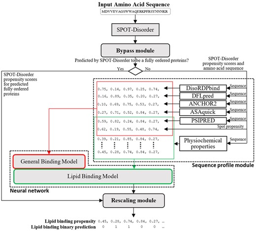
Prediction workflow of DisoLipPred.
2.3.1 Bypass module
DLBRs are localized in the disordered regions. The main challenge for DisoLipPred is to identify these lipid-binding residues among the other disordered residues. Consequently, during the training process we train and validate the deep network on the native disordered residues. We exclude the ordered residues from training since they can be accurately identified with one of the currently available accurate disorder predictors. We use the highly accurate SPOT-Disorder predictor (Hanson et al., 2017) for that purpose. The bypass module separates disordered residues from ordered residues based on the SPOT-Disorder’s predictions, such that the putative ordered residues bypass the prediction process while the putative disordered residues are selected for prediction with the deep network. The SPOT-Disorder generated propensities for the putative ordered residues are rescaled and combined with the deep network generated propensities in the rescaling module to produce the propensities for DLBRs. We use ablation analysis (Section 3.1) to demonstrate that the approach that applies the bypass module provides more accurate results than the direct prediction of DLBRs from all residues.
2.3.2 Sequence profiles
The sequence profiles provide a rich source of information that is relevant to the prediction of DLBRs and derived directly from the sequences. We use two profiles to facilitate the transfer learning. One for the partner–agnostic portion of the deep network that aims to predict interacting disordered residues (red areas in Fig. 1) and the other for the part of the deep network that predicts DLBRs (green areas in Fig. 1).
The partner–agnostic profile relies on a comprehensive collection of predictors of structure, intrinsic disorder and disorder functions, with particular focus on the prediction of the interacting disordered regions. We use the predictions of the solvent accessibility from ASAquick (Faraggi et al., 2014), secondary structure from PSIPRED (Buchan et al., 2013), disorder from SPOT-Disorder (Hanson et al., 2017), protein, DNA and RNA interacting disordered regions from DisoRDPbind (Peng et al., 2017; Peng and Kurgan, 2015), protein-binding disordered regions from ANCHOR 2 (Mészáros et al., 2018) and disordered linker regions from DFLpred (Meng and Kurgan, 2016). This profile is summarized in Supplementary Table S2.
The second profile, which serves as the input to predict DLBRs, focuses on the sequence-derived information that is specific to the lipid-binding. We use two relevant structural properties, the putative solvent accessibility and secondary structure generated with ASAquick (Faraggi et al., 2014) and PSIPRED (Buchan et al., 2013), respectively, putative disorder from SPOT-Disorder (Hanson et al., 2017), and a curated set of 46 physiochemical properties of amino acids that are associated with protein–lipid interactions (Huang et al., 2013). These properties were selected empirically from a comprehensive collection of over 530 physiochemical indices from the AAindex database (Kawashima et al., 2008) based on their ability to discriminate between lipid-binding and non-lipid binding proteins (Huang et al., 2013). They include hydrophobicity, hydrophobic moment, charge, isoelectric point, transfer energy, activation Gibbs energy of unfolding at pH 9.0, solvation free energy, propensity for helical and sheet conformations, and propensity for side chain interactions. Complete list of these properties is in Supplementary Table S3.
2.3.3 Transfer learning of the deep bidirectional recurrent neural network model
Transfer learning is a training strategy where knowledge learned from a source domain/dataset is transferred to a related target domain/dataset to improve the learning in the target domain (Weiss et al., 2016). This strategy is deployed when the target dataset has limited amount of data compared to a more data-rich source dataset, and is particularly useful for training the data-hungry deep neural networks (Tan et al., 2018). Transfer learning was recently applied to predict secondary structures of RNA (Singh et al., 2019), caspase and metalloprotease cleavage sites (Li et al., 2020), MHC‐I peptide binding (Jin et al., 2021) and transcription factor binding (Liu et al., 2021), but it was never used to develop predictors of interacting disordered regions. Prediction of DLBRs offers an ideal scenario for the transfer learning. While we have a relatively limited amount of DLBRs (3392 residues), the amount of the data concerning a generic set of interacting IDRs is very substantial (161 641 residues). Thus, we first build a partner–agnostic deep network using the complete training dataset, which we then freeze and extend with additional layers to develop the target network that predicts DLBRs using the target training dataset. We adopt deep recurrent networks given their recent success with the prediction of disorder (Hanson et al., 2017, 2018, 2020,b).
The partner–agnostic network consists of two long short-term memory layers that are sandwiched between fully connected dense layers with ReLu activation function in the internal layers and the sigmoid activation function at the output layer (Supplementary Fig. S2A). We use the RMSprop optimizer, binary cross entropy as the loss function, dropout rate of 0.5 (to minimize overfitting), and dynamic adjustment of the learning rate which we set to gradually decrease as the training progresses. This network uses the partner–agnostic profile as the input. We optimized the number of layers and the number of neurons per layer using an iterative approach where we start from a small size and increase it by a small increment until AUC measured for the prediction of interacting IDRs on the validation set decreases in two consecutive iterations.
The optimized partner–agnostic network is transferred to develop the target network. We remove the output layer from the partner–agnostic model and freeze it. We connect the last layer of this network to several additional layers that narrow down the partner–agnostic prediction to the partner-specific prediction of DLBRs. This network extends the partner–agnostic profile with the additional inputs relevant to the prediction of DLBRs that we discuss in Section 2.3.2. This extension includes multiple bidirectional long short-term memory layers placed between fully connected dense layers (Supplementary Fig. S2B). Similar to the training of the partner–agnostic network, we optimize the size of the additional layers using the increment approach that maximizes AUC for the prediction of DLBRs on the validation set.
2.3.4 Rescaling module
We combine the disordered lipid-binding propensities generated by our deep recurrent neural network for the disordered residues predicted with SPOT-Disorder and the SPOT-Disorder’s propensity scores for the predicted ordered residues. First, we normalize the outputs from the deep neural network to the unit range. We also rescale the SPOT-Disorder’s propensities for predicted ordered residues, which bypass the neural network, so they cover the 0–0.5 range. This aims to minimize risk of missing out the lipid-binding residues among the incorrect predictions of order from SPOT-Disorder. This way, these false negatives can be predicted with moderately high scores.
3 Results
3.1 Ablation analysis
The three main innovations underlying DisoLipPred include the use of the transfer learning, lipid-binding features and the bypass module. We perform ablation analysis to quantify the impact of these innovations on the predictive performance of DisoLipPred. To do that, we compare the results produced by the DisoLipPred model with the three setups where one of these features is removed and the setup where all three features are removed (Table 1). For instance, in the setup 1 we exclude transfer learning by removing the partner–agnostic network and relying solely of the lipid binding neural network. The bypass module works by training and testing the deep network on the disordered residues and sidestepping the deep network predictions for the putative ordered residues. The training process utilizes the native disordered residues while during tests/predictions we use the predictions from SPOT-Disorder. In setup 3, we evaluate the impact of using the predicted disordered residues for both training and testing/predictions. The setup 4 excludes all three innovations where for the bypass feature we train/test the deep network using both disordered and ordered residues. This bare-bone predictor is comparable to current deep learners that are used to predict disorder (Hanson et al., 2017, 2020,b; Wang et al., 2016,b) and the protein binding IDRs (Fang et al., 2019; Hanson et al., 2020a). We trained each of the five setups separately by maximizing the AUC on the validation set.
Experimental setups for the ablation study
| Setup | Use of transfer learning | Use of lipid features | Bypass module during training |
|---|---|---|---|
| DisoLipPred | Yes | Yes | Native disorder versus native order |
| 1 | No | Yes | Native disorder versus native order |
| 2 | Yes | No | Native disorder versus native order |
| 3 | Yes | Yes | Predicted disorder versus predicted order |
| 4 | No | No | No |
We compare predictive performance of the five setups on the test dataset in Table 2. Supplementary Table S4 compares these methods on the validation dataset. Both tables assess the predictions on the complete datasets as well as on the subset of the disordered residues. The latter evaluation quantifies the ability of these models to solve a more difficult problem of identifying DLBRs among other disordered regions i.e. DLBR are more similar to other disordered residues than to the ordered residues.
Predictive performance of DisoLipPred and its variants from the ablation analysis (Table 1) on the test dataset
| Setup | Complete dataset | Disordered residues in the test dataset | ||||||||||||||||
|---|---|---|---|---|---|---|---|---|---|---|---|---|---|---|---|---|---|---|
| AUC | Spec = 0.90 | Spec = 0.70 | Sens = 0.70 | Sens = 0.50 | AUC | Spec = 0.90 | Spec = 0.70 | Sens = 0.70 | Sens = 0.50 | |||||||||
| Sen | F1 | Sen | F1 | Spec | F1 | Spec | F1 | Sen | F1 | Sen | F1 | Spec | F1 | Spec | F1 | |||
| DisoLipPred | 0.781 | 0.382 | 0.145 | 0.745 | 0.111 | 0.731 | 0.115 | 0.831 | 0.124 | 0.635 | 0.286 | 0.201 | 0.500 | 0.161 | 0.465 | 0.138 | 0.699 | 0.161 |
| 1 | 0.747 | 0.290 | 0.112 | 0.287 | 0.044 | 0.278 | 0.047 | 0.492 | 0.047 | 0.572 | 0.162 | 0.118 | 0.469 | 0.151 | 0.438 | 0.133 | 0.666 | 0.148 |
| 2 | 0.745 | 0.327 | 0.125 | 0.154 | 0.024 | 0.234 | 0.044 | 0.370 | 0.038 | 0.603 | 0.146 | 0.175 | 0.421 | 0.142 | 0.430 | 0.130 | 0.564 | 0.132 |
| 3 | 0.726 | 0.260 | 0.101 | 0.296 | 0.046 | 0.344 | 0.051 | 0.513 | 0.049 | 0.593 | 0.117 | 0.129 | 0.326 | 0.108 | 0.369 | 0.121 | 0.552 | 0.116 |
| 4 | 0.678 | 0.123 | 0.049 | 0.418 | 0.064 | 0.506 | 0.067 | 0.650 | 0.066 | 0.396 | 0.046 | 0.035 | 0.201 | 0.068 | 0.181 | 0.096 | 0.352 | 0.086 |
Note: We perform the assessment on the complete test dataset, and also on the subset of disordered residues from the test dataset. We quantify the binary metrics (sensitivity, specificity and F1) at fixed sensitivities (sens) of 0.70 and 0.50 and fixed specificities (spec) of 0.90 and 0.70. This enables direct comparison of the binary metrics between different variants. We assess the statistical significance of the differences between the results produced by DisoLipPred and each of the variants using procedure explained in Section 2.2. Values in bold and italics font indicate that DisoLipPred provides significantly better result when compared with its variant (P-value <0.05).
DisoLipPred offers accurate predictions with AUC = 0.78 and high sensitivity and specificity values. We calibrate the binary predictions based on thresholds that fix sensitivity to 0.70 and 0.50 and that fix specificity to 0.90 and 0.70. This facilitates direct comparison of sensitivity, specificity and F1 values between different setups. Compared to the complete DisoLipPred model, we note a noticeable and statistically significant drop in the predictive performance for all metrics and ablation variants (P-value < 0.05). Among the setups where one of the innovations is removed, the largest drop is for the setup 3 where we manipulate the bypass feature. This suggests that our deep networks can be better trained to recognize DLBR among native disordered residues than among the predicted disordered residues. The errors from the disorder predictions and the networks training seem to accumulate in the latter case. The results further substantially decline when all three innovations are removed (setup 4). This means that the contributions of the novel design features are complementary.
As expected, tests on the native disordered residues (right side of Table 2) lead to lower predictive performance across all methods. However, DisoLipPred still provides reasonably accurate predictions (AUC = 0.64 and substantially higher sensitivity and specificity valulues). The ablation variants consistently underperform compared to the complete model (P-value < 0.05), with the bare-bone model (setup 4) performing at the random levels: AUC < 0.5 and sensitivity, specificity and F1 near zero. This demonstrates that the basic deep network is incapable of predicting DLBRs since it can only solve the trivial problem of differentiating DLBRs from ordered residues (AUC = 0.68 on the complete dataset versus 0.40 on the disordered residues). In other words, the three innovations that we introduce are essential to provide accurate predictions.
3.2 Comparative assessment on the test dataset
We compare DisoLipPred to current alternatives that can be indirectly used to predict DLBR. We consider three categories of the indirect predictors. First, we include methods that predict transmembrane regions in protein sequences. We select predictors with publicly available implementations/servers that include one recently released method, SCAMPI 2 (Peters et al., 2016) and one older and highly cited method, Phobius (Käll et al., 2007). While DLBRs predicted by DisoLipPred exclude transmembrane regions, we investigate whether the transmembrane region predictors could be used to also predict DLBRs. Second, we cover disorder predictors since DLBR are one of the functional subtypes of the disordered residues. We choose 10 disorder predictors that were considered in recent comparative surveys (Katuwawala et al., 2020; Katuwawala and Kurgan, 2020): DisEMBL‐465 (trained using X‐ray structures) and DisEMBL‐HL (trained to predict disorder-like loop conformations) (Linding et al., 2003); three versions of ESpritz (Walsh et al., 2012): ESpritz‐Xray (trained on X‐ray structures), ESpritz‐NMR (trained on NMR structures) and ESpritz‐DisProt (trained on the DisProt database data); two flavors of IUPred (Dosztányi et al., 2005; Mészáros et al., 2018): IUPred‐short (trained to predict short IDRs) and IUPred‐long (trained to predict long IDRs); GlobPlot (Linding et al., 2003) and SPOT-Disorder (Hanson et al., 2017). Third, we include representative predictors of disorder function, such as DisoRDPbind (Peng et al., 2017; Peng and Kurgan, 2015) that predicts the disordered RNA binding, DNA binding and protein binding residues, ANCHOR 2 (Mészáros et al., 2018) that predicts disordered protein binding residues and DFLpred (Meng and Kurgan, 2016) which predicts disordered linkers. Finally, we compute a baseline results based on sequence alignment to the training proteins. We perform this alignment with BLAST (Altschul et al., 1997), where DLBR annotations are transferred from the aligned positions in the most similar training proteins that secures e-value < 1.0. We setup the e-value parameter to maximize performance on the test dataset.
Table 3 compares DisoLipPred’s predictive performance against the indirect predictors and the baseline. We derive the binary predictions from the propensity scores using thresholds that we adjust to set FPR = 0.1 (specificity = 0.9). This allows us to directly compare the other binary metrics (sensitivity and F1) between methods. DisoLipPred provides accurate predictions of DLBRs on the test dataset, with AUC = 0.78 and sensitivity = 0.38 at FPR = 0.10. The latter means that DisoLipPred offers 3.8-fold increase in the rate of correct to incorrect predictions. Tests of statistical significance of differences reveal that the DisoLipPred’s predictions are significantly better than the results of all 17 indirect methods and the baseline (P-value < 0.05). The poor performance of the baseline alignment stems from the low sequence similarity, < 25%, between the training and test proteins. The most accurate of the indirect predictors include Espritz-DisProt (AUC = 0.77, sensitivity = 0.35), SPOT-Disorder (AUC = 0.69, sensitivity = 0.16) and VSL2B (AUC = 0.67, sensitivity = 0.21). The ROC curves the test dataset for the best-performing methods, including DisoLipPred, SPOT-Disorder, VSL2B, Espritz-DisProt, are available in Supplementary Figure S3. They reveal a large margin of improvement for DisoLipPred, particularly for low values of FPRs, i.e. conservative predictions where rate of false positives is low. We highlight the results from the two predictors of transmembrane regions that secure near zero (0.02) sensitivity at 0.1 specificity, which means that they do not predict DLBRs. We further investigate these methods using a dataset of transmembrane proteins in Section 3.4.
Predictive performance on the test dataset
| Predictor | Complete test dataset | Disordered residues in the test dataset | |||||||
|---|---|---|---|---|---|---|---|---|---|
| Type | Name | AUC | Sensitivity | F1 | Specificity | AUC | Sensitivity | F1 | Specificity |
| Transmembrane regions | SCAMPI 2 | N/A | 0.019 | 0.016 | 0.98 | N/A | 0.019 | 0.035 | 0.99 |
| Phobius | N/A | 0.016 | 0.024 | 1.00 | N/A | 0.016 | 0.031 | 1.00 | |
| Baseline | BLAST alignment | N/A | 0.000 | 0.000 | 1.00 | N/A | 0.000 | 0.000 | 1.00 |
| Disorder function predictors | DFLpred | 0.338 | 0.037 | 0.015 | 0.90 | 0.554 | 0.109 | 0.081 | 0.90 |
| DisoRDPbind-RNA | 0.450 | 0.035 | 0.014 | 0.90 | 0.517 | 0.028 | 0.022 | 0.90 | |
| ANCHOR | 0.637 | 0.229 | 0.090 | 0.90 | 0.446 | 0.178 | 0.129 | 0.90 | |
| DisoRDPbind-Protein | 0.556 | 0.016 | 0.006 | 0.90 | 0.276 | 0.002 | 0.001 | 0.90 | |
| DisoRDPbind-DNA | 0.636 | 0.211 | 0.083 | 0.90 | 0.554 | 0.062 | 0.047 | 0.90 | |
| Disorder predictors | GlobPlot | 0.530 | 0.225 | 0.088 | 0.90 | 0.482 | 0.167 | 0.123 | 0.90 |
| ESpritz-NMR | 0.571 | 0.216 | 0.085 | 0.90 | 0.412 | 0.113 | 0.084 | 0.90 | |
| disEMBL-465 | 0.610 | 0.119 | 0.048 | 0.90 | 0.433 | 0.048 | 0.037 | 0.90 | |
| disEMBL-HL | 0.619 | 0.143 | 0.056 | 0.90 | 0.477 | 0.066 | 0.050 | 0.90 | |
| IUPred-long | 0.626 | 0.256 | 0.100 | 0.90 | 0.420 | 0.167 | 0.123 | 0.90 | |
| IUPred-short | 0.632 | 0.257 | 0.100 | 0.90 | 0.441 | 0.142 | 0.105 | 0.90 | |
| ESpritz-Xray | 0.659 | 0.114 | 0.046 | 0.90 | 0.428 | 0.070 | 0.053 | 0.90 | |
| VSL2B | 0.673 | 0.205 | 0.081 | 0.90 | 0.433 | 0.057 | 0.045 | 0.90 | |
| SPOT-Disorder | 0.692 | 0.155 | 0.062 | 0.90 | 0.361 | 0.043 | 0.033 | 0.90 | |
| ESpritz-DisProt | 0.768 | 0.355 | 0.135 | 0.90 | 0.498 | 0.065 | 0.049 | 0.90 | |
| DLBR predictor | DisoLipPred | 0.781 | 0.382 | 0.145 | 0.90 | 0.635 | 0.286 | 0.201 | 0.90 |
Note: We perform the assessment on the complete test dataset, and also on the subset of the native disordered residues from the test dataset. We quantify the binary metrics (sensitivity and F1) at the fixed specificity = 0.9 for the predictors that produce the propensity scores. We use the default sensitivity, F1 and specificity values for the other three methods that produce only binary predictions: SCAMPI 2, Phobius and BLAST. We assess the statistical significance of the differences between the results produced by DisoLipPred and every other tool using procedure explained in Section 2.2. Values in bold and italics font indicate that DisoLipPred provides significantly better results when compared with a given other predictor (P-value <0.05). Methods are sorted in the ascending order by their AUC within each predictor type group.
The prediction of DLBRs requires to separate these residues from structured residues and from other disordered residues. The first task of differentiating disorder from order can be solved accurately by current methods, as demonstrated by recent assessments of disorder predictors (Katuwawala and Kurgan, 2020; Necci et al., 2021). This is why several disorder predictors secure relatively high AUCs of on the test dataset. The second task is hard, which is apparent from the results computed on the native disordered residues in the test dataset (the right side of Table 3). They reveal that disorder predictors cannot reliably discriminate DLBRs from the other disordered residues, which is expected since they were not designed for this prediction. More specifically, AUCs of the top disorder predictors, Espritz-DisProt, SPOT-Disorder, VSL2B, are 0.50, 0.36 and 0.43, respectively. Some of these AUCs are substantially below 0.5, suggesting that the scores for the DLBRs are lower than for the other disordered residues. This could be explained by the fact that DLBRs fold upon binding, therefore having higher propensity to be structured from some other disordered residues. However, the ability to use these predictions to find DLBRs would hinge on first correctly predicting disordered residues. Only DisoLipPred solves the hard prediction by producing relatively accurate results for the disordered residues (AUC = 0.64, F1 = 0.20 and sensitivity = 0.29 at specificity = 0.90), with the other predictors scoring at random levels (AUCs ≤ 0.55) and these differences being statistically significant (P-value < 0.05).
3.3 Predictions on the Saccharomyces cerevisiae proteome
We apply DisoLipPred to predict DLBRs for the complete Saccharomyces cerevisiae proteome that we source from UniProt (UniProt, 2021). The Baker’s yeast proteome includes 6049 protein sequences and 2 936 363 residues. This is one of the most accurately sequenced proteomes; BUSCO (Benchmarking Universal Single-Copy Orthologs) scores its completeness at 99.6% (Simão et al., 2015). We calibrate the binary predictions to 0.48% prediction rate (% putative DLBRs in the genome), which corresponds to the rate of the native DLBRs in the DisProt database. We exclude the putative DLBRs if they form segments of <6 consecutive residues since the shortest experimentally annotated disordered lipid binding regions in DisProt are 6 residues long. We share these predictions on the DisoLipPred’s website at http://biomine.cs.vcu.edu/servers/DisoLipPred/. We predict that about 4.9% of the yeast proteins have putative DLBRs (Fig. 2A). Majority of these proteins have less than 5% of residues predicted as DLBRs, however, about 0.7% of the yeast proteins have a substantial amount of over 5% DLBRs (Fig. 2B).
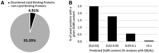
Summary of the DisoLipPred’s predictions on the Saccharomyces cerevisiae proteome. (A) The fraction of the yeast proteins predicted to have DLBRs. (B) The histogram of the putative content of DLBRs for the 4.9% of the yeast proteins with DLBRs
We validate these predictions using the gene ontology (GO) annotations from UniProt. These annotations are independent of the ground truth data used in the test dataset. First, we select a subset of the yeast proteins that include the ‘lipid’ keyword in their molecular function GO term and the ‘membrane’ keyword within their cellular component GO term. The resulting set of 309 proteins is likely to be enriched in the proteins that have DLBRs; we call it GO lipid associated protein set. Second, we compute the rate of proteins predicted to have DLBRs in the GO lipid associated protein set using DisoLipPred and compare it to the rate of these predictions generated with the second-best ESpritz-DisProt method (Table 2). We calibrate the ESpritz-DisProt’s predictions the same way as the predictions from DisoLipPred. Third, we calculate the expected rate of proteins with the putative DLBRs in the yeast proteome. We compute the rate for a randomly selected set of 309 yeast proteins and repeat this experiment 100 times to establish distribution of the expected rates. The results are summarized in Figure 2. The mean of the distribution for DisoLipPred’s predictions is 4.9% (Fig. 3A) and corresponds to the overall rate of proteins with DLBRs in yeast (Fig. 2A).
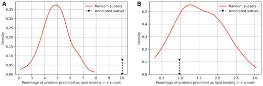
Analysis of the DisoLipPred predictions (A) and the Espritz-DisProt predictions (B) for the yeast proteins. The black arrows identify the rate of the putative proteins with DLBRs in the GO lipid associated protein set (i.e. set of 309 yeast proteins that share ‘lipid’ keyword in the molecular function GO term and the ‘membrane’ keyword in the cellular component GO term). Red lines show the distributions of the expected rates of the putative proteins with DLBRs, which we establish based on measuring the rate for 100 randomly selected sets of 309 yeast proteins (Color version of this figure is available at Bioinformatics online.)
DisoLipPred predicts 10.3% of proteins in the GO lipid associated protein set as having DLBRs. This rate doubles the expected rate of 4.9% and the difference is statistically significant based on the distribution of the expected values in Figure 3A (P-value < 0.01). On the other hand, the calibrated predictions from ESpritz‐DisProt identify only 0.97% of the GO lipid associated protein set as having DLBRs. This rate is below the expected rate of the ESpritz‐DisProt’s predictions (red line in Fig. 3B), for which median is 1.5%. This suggests that the GO lipid associated proteins are overall depleted in disorder. In spite of the disorder depletion, the rate of the DisoLipPred’s predictions of DLBRs is 10.3/0.97 = 10.6 times higher than the rate of the ESpritz‐DisProt’s predictions, providing further support for our claim that DisoLipPred’s predictions are accurate.
3.4 Assessment of predictions on the transmembrane proteins
Given that DLBR are defined as disordered lipid-binding regions that exclude transmembrane segments, we empirically evaluate whether the DisoLipPred’s predictions in fact exclude the transmembrane residues. We test DisoLipPred and the two representative predictors of the transmembrane regions, SCAMPI 2 (Peters et al., 2016) and Phobius (Käll et al., 2007), on the TM dataset (Table 4). Here, we use the predictions from these three tools to identify native transmembrane regions, i.e. transmembrane residues are set as the positives while the other residues, including a small amount of DLBRs, are set as negatives. Since SCAMPI 2 and Phobius produce only binary predictions and thus their prediction rate cannot be calibrated, we adjust the rate of the DisoLipPred’s predictions to match the specificity of each of the two transmembrane predictors. Table 4 shows that as expected SCAMPI 2 and Phobius provide accurate predictions of the transmembrane regions based on their high sensitivity scores, i.e. 0.79 sensitivity at the low 0.09 FPR and 0.57 sensitivity at the low 0.06 FPR, respectively. Their predicted positive rate (PPR) defined as the rate of true positives among the predicted positives is also relatively high and equals 0.28 and 0.20, respectively. In stark contrast, DisoLipPred’s sensitivity values calibrated to the rate of predictions from SCAMPI 2 and Phobius are 0.04 and 0.03, demonstrating that it predicts very few transmembrane resides as DLBRs. These values are substantially smaller than the corresponding sensitivity values on the test dataset (Supplementary Fig. S3). DisoLipPred’s PPR is higher than its corresponding sensitivity because several proteins in this dataset include DLBRs, which by definition do not overlap with transmembrane regions. Altogether, these results show that DisoLipPred accurately differentiates between the transmembrane regions and DLBRs. Moreover, given the correspondingly low sensitivity of SCAMPI 2 and Phobius for the prediction of DLBRs (Table 3), we conclude that DisoLipPred predicts lipid interacting residues that complement the results produced by the predictors of the transmembrane regions.
Predictive performance on the TM dataset
| Predictor | Sensitivity | Specificity | PPR | F1 |
|---|---|---|---|---|
| SCAMPI 2 | 0.795 | 0.91 | 0.279 | 0.780 |
| DisoLipPred at | 0.041 | 0.91 | 0.076 | 0.063 |
| SCAMPI 2 specificity | ||||
| Phobius | 0.574 | 0.94 | 0.197 | 0.663 |
| DisoLipPred at | 0.035 | 0.94 | 0.050 | 0.059 |
| Phobius specificity |
Note: The performance is measured assuming that the native transmembrane regions constitute positive annotations. Both transmembrane predictors (SCAMPI 2 and Phobius) produce only binary predictions and thus their prediction rate cannot be calibrated. Instead, we calibrate the rate of the DisoLipPred’s predictions to match the specificity of SCAMPI 2 and Phobius.
3.5 Case study
We illustrate the DisoLipPred’s predictions for one of the test proteins, the Sec-independent protein translocase protein TatA (UniProt accession number: P69428). Our objective here is to visualize and explain the predictions, rather than to evaluate their performance. TatA is a membrane associated protein, which is a subunit of the larger twin-arginine translocation (Tat) system (Chan et al., 2011). The Tat system acts as a facilitator to transport large folded proteins through cellular membranes by creating a protein conducting channel (Ize et al., 2002; Sargent et al., 1998). TatA contains a long IDR (positions 21–89) which was characterized with NMR (Zhang et al., 2014). Furthermore, proton based NMR revealed that part of this IDR (positions 21–44) binds to lipids (Chan et al., 2011). Figure 4 shows DisoLipPred’s predictions for TatA along with the abovementioned native annotations of the disordered and disorder lipid binding regions. DisoLipPred generates relatively high propensities at the N terminus half of the protein, resulting in the prediction of a long segment of DLBRs that overlaps with the experimentally determined lipid-binding region. Interestingly, we predict that the residues at the N terminus are also lipid binding. DisProt does not offer a conclusive evidence whether this segment is disordered or structured. Our alignment-based mapping into PDB (see Section 2.1) did not identify a known structure for this segment. Further investigation of literature reveals support for our prediction, where this segment is shown to likely interact with lipids of the cell membrane from the cytoplasmic side (Porcelli et al., 2002). Altogether, this prediction agrees with the experimental annotations and provides support for the hypothesis that the disordered lipid binding region is larger than DisProt suggests, covering the N-terminus half of the TatA sequence.
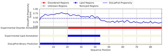
DisoLipPred predictions for TatA protein (Uniprot: P69428; DisProt: DP00834). The blue line in the top panel shows the residue level propensity scores generated by DisoLipPred. The horizontal blue bars at the bottom are the corresponding experimental annotation of lipid binding regions and the binary prediction from DisoLipPred. The horizontal red bar shows the experimental annotation of the intrinsic disorder, where gray color identifies regions that lack disorder/order annotations
3.6 Webserver
DisoLipPred is freely available as a webserver at http://biomine.cs.vcu.edu/servers/DisoLipPred/. DisoLipPred webserver takes up to two amino acid sequences in the FASTA format as the input. The entire prediction process is automated, done on the server side and takes about 2–4 min for an average size protein. Users can optionally provide an email address where we send a notification email with the unique URL of results once the prediction is completed. The webserver provides the output propensities and binary predictions for each amino acid in the input protein sequence(s). The threshold that we use to generate the binary predictions corresponds to the 10% FPR on the training dataset. The outputs are available in two complementary formats: as a parsable text file and an interactive figure. The figure provides a graphical summary of the predictions with the zoom in/out functions, ability to hide user-selected panels and take a screenshot and mouse hover that shows additional information.
4 Summary
IDRs interact with many partner molecules including proteins, RNA, DNA and lipids. Sequence-based prediction of these IDRs is currently possible for the interactions with proteins and nucleic acids (Katuwawala et al., 2019a,b; Meng et al., 2017; Varadi et al., 2015a). Motivated by the growing amount of experimental data and the need to expand coverage of the current predictors, we conceptualize, design, validate and deploy DisoLipPred, the first predictor of DLBRs. Our solution implements three innovative features that include the application of transfer learning, bypass module and selected physiochemical properties associated with protein–lipid interactions.
We deliver a multifaceted validation of the predictions produced by DisoLipPred. The ablation tests show that the quality of the DisoLipPred predictions is powered primarily by the three innovations. Analysis on the test dataset reveals that DisoLipPred generates accurate predictions and that current tools that could be indirectly used to identify DLBR cannot differentiate the lipid-interacting residues from the other disordered residues. Validation on the complete yeast proteome provides further support for the claim that DisoLipPred produces accurate results. Moreover, we demonstrate empirically that the DisoLipPred’s predictions complement the results produced by the predictors of the transmembrane regions. Altogether, our analysis suggests that DisoLipPred provides high-quality predictions of disordered lipid-binding regions that complement the currently available tools. DisoLipPred is available via a convenient webserver at http://biomine.cs.vcu.edu/servers/DisoLipPred/.
Funding
This research was supported in part by the National Science Foundation [1617369] and the Robert J. Mattauch Endowment funds.
Conflict of Interest: none declared.

