DULoc: quantitatively unmixing protein subcellular location patterns in immunofluorescence images based on deep learning features

Abstract

Motivation

Knowledge of subcellular locations of proteins is of great significance for understanding their functions. The multi-label proteins that simultaneously reside in or move between more than one subcellular structure usually involve with complex cellular processes. Currently, the subcellular location annotations of proteins in most studies and databases are descriptive terms, which fail to capture the protein amount or fractions across different locations. This highly limits the understanding of complex spatial distribution and functional mechanism of multi-label proteins. Thus, quantitatively analyzing the multiplex location patterns of proteins is an urgent and challenging task.

Results

In this study, we developed a deep-learning-based pattern unmixing pipeline for protein subcellular localization (DULoc) to quantitatively estimate the fractions of proteins localizing in different subcellular compartments from immunofluorescence images. This model used a deep convolutional neural network to construct feature representations, and combined multiple nonlinear decomposing algorithms as the pattern unmixing method. Our experimental results showed that the DULoc can achieve over 0.93 correlation between estimated and true fractions on both real and synthetic datasets. In addition, we applied the DULoc method on the images in the human protein atlas database on a large scale, and showed that 70.52% of proteins can achieve consistent location orders with the database annotations.

Availability and implementation

The datasets and code are available at: https://github.com/PRBioimages/DULoc.

Supplementary information

Supplementary data are available at Bioinformatics online.

1 Introduction

Proteins are found in various subcellular compartments with specific chemical environments, which can provide clues for their functions, interactions and molecular mechanisms. Automated recognition of protein subcellular location patterns has been an important part of bioinformatics over the past decades (Rastogi and Rost, 2010; Thul et al., 2017). As many proteins show highly complex location patterns in human cells, the recognition task is still challenging. Over half of human proteins reside in more than one subcellular structure. These proteins are called multi-label proteins (Chou and Shen, 2010; Simha et al., 2015; Stadler et al., 2013), and many of their translocations within cells involve with diseases, such as metabolic, cardiovascular, neurodegenerative diseases and cancers (Hung and Link, 2011). These translocations refer to the change of subcellular location, amount or fraction of proteins. Thus, pinpointing the subcellular locations and quantifying distribution fractions of these multi-label proteins can significantly expand our knowledge of them and help in disease diagnosis and treatments.

Compared with amino acid sequences, bioimages can intuitively show protein spatial distribution and variation, and are suitable for location analysis. Immunofluorescence (IF) microscopy imaging, as a low-cost and high-efficiency biotechnology, has gained increasing popularity in automated analysis of protein location patterns (Barbe et al., 2008; Fagerberg et al., 2011). Currently, most of the studies about protein subcellular localization are qualitative classification. The methods mainly include traditional feature engineering (Boland et al., 1998; Murphy et al., 2000) and deep learning (Kraus et al., 2017; Long et al., 2020; Nanni et al., 2019; Pärnamaa and Parts, 2017), where the latter has achieved impressive performance in recent years. For example, a convolutional neural network (CNN) model called bestfitting, which was trained based on DenseNet (Huang et al., 2017), got a macro F1 score of 0.593 over 28 subcellular classes, and won the first prize in a worldwide competition of protein localization classification (Ouyang et al., 2019).

To date, there are only a few works that tried to quantitatively estimate the fractions of protein distribution in various subcellular organelles. One reason is the lack of labeled data. The human protein atlas (HPA, https://proteinatlas.org) database stores tens of thousands of IF images of human proteins, but the subcellular location annotations for these images are descriptive terms without quantitative information. For this problem, Murphy group generated a quantitatively labeled dataset of fluorescent images using molecular probes to control mitochondrial and lysosomal concentration fractions (Peng et al., 2010). Based on this dataset, they developed automated unmixing models to map the amount of fluorescence to quantitative fractions (Coelho et al., 2010; Peng et al., 2010; Zhao et al., 2005). The models used morphological and texture features to describe fluorescent objects in images and clustered all the objects, thus each image was represented by the object frequencies across the clusters. Then the patterns of multi-label proteins were regarded as linear mixtures of fundamental single-label patterns, and were resolved by linear unmixing algorithms. Besides, Yang et al. assumed that the pattern unmixing was a nonlinear problem, and proposed to use nonlinear regression method to unmix the protein patterns (Yang et al., 2016). They employed a variable-weighted support vector machine (VW-SVM) model optimized by particle swarm optimization, and demonstrated that nonlinear techniques could achieve better performance in this task.

These works have provided useful strategies for protein quantitative analysis, but there still exist some limitations. First, the protein patterns were represented by only fluorescent object features in these methods. Considering the remarkable representation power of CNNs, more accurate descriptors should be adopted. Second, due to the constraint of quantitatively labeled data, the unmixing was only performed on two subcellular location classes, i.e. mitochondrion and lysosome. The VW-SVM model could not be extended to other classes because the training process requires lots of mixed data labeled with fraction annotations. Therefore, it is necessary to develop new models with high accuracy and better applicability for protein subcellular location pattern unmixing.

In this study, we proposed a new deep-learning-based unmixing method, called DULoc, to quantify the fractions of protein distribution in subcellular compartments. The DULoc has two core modules, where the first one used the bestfitting network to construct a feature space for IF images, and the second utilized a combined nonlinear approach to decompose the mixed patterns. The model did not need large amount of quantitatively labeled data to train, and it was tested effective on the real labeled dataset, a synthetic dataset and a large-scale quantitative analysis of images in the HPA database.

2 Materials and methods

2.1 Datasets

There were two datasets used during the construction of our unmixing models (Fig. 1).

Fig. 1.

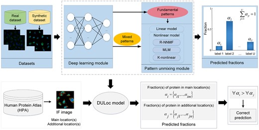
Flowchart of the experiments in this article. There are two sections, i.e. the construction of DULoc model and its application. In the first section, the fluorescence images were processed by the deep learning module to extract subcellular pattern features. The fundamental patterns are the patterns of single-location proteins and the mixed patterns are those of multi-label proteins. Each mixed pattern was decomposed by the pattern unmixing module to get fractions. The unmixing module was tested on a real and a synthetic dataset, and the final DULoc was constructed according to their results. In the second section, the IF images with qualitative annotations from the HPA database were fed into the DULoc to get the fractions of proteins across the annotated subcellular locations. Evaluation of the fractions was based on the fact that each of the annotated subcellular locations for one image was manually assigned as either main or additional in the HPA. If all of the fraction(s) of protein in main location(s) are higher than those of additional location(s), the image would be regarded as a correct prediction. The consistency between the predicted fractions and the order of qualitative annotations was used as the evaluation criterion of the large-scale application

2.1.1 Real dataset

The first dataset was the fluorescence image dataset constructed by Murphy group (Peng et al., 2010). The dataset consisted of 64 groups of high-throughput microscopy images, where each group was labeled with a specific mixture fraction of fluorophore-tagged mitochondrial and lysosomal probes. The total number of images in the real dataset is 2056, and each image has nucleus and protein channels. The advantage of the real dataset is that the quantitative annotations are true and reliable, while the limitation is that there are only two labels assigned.

2.1.2 Synthetic dataset

As the fact that the real dataset only has two classes limits the generalization of unmixing algorithms for multi-label proteins, we tried to synthesize a new dataset with various mixed patterns. The steps of the image synthesis process are shown in Figure 2. First, 1648 IF images of the U-2 OS cell line that were annotated with one of five major subcellular locations, i.e. cytosol, nucleoplasm, plasma membrane, nucleoli and mitochondria, were selected from the HPA database. Each image has four channels, i.e. protein (green), nucleus (blue), ER (yellow) and microtubule (red). All of the images were annotated with enhanced or supported reliability in the database and can be regarded as pure fundamental patterns. Using cell masks provided by the HPA database, the images were segmented into single cells. Nucleus regions were also segmented by morphological operations to outline contours of the nuclei. Then, the subsequent processing for the segmented cells included rotating to make the long axis of nuclei horizontally and padding. This was to facilitate the matching of cells of different patterns. Pairs of regions that have over 90% overlap in nucleus masks and over 75% overlap in cell masks were selected to conduct cell mergence. The mergence assumed that a mixed subcellular location pattern was approximately the weighted sum over fundamental patterns. The cells of mixed patterns were generated with five concentration fractions, i.e. 0:1, 0.25:0.75, 0.5:0.5, 0.75:0.25 and 1:0 between two fundamental patterns. In addition, considering that the difference of IF image intensity between two images had impact on the protein quantitation, we adjusted the gray levels of images in mixed regions into similar distribution by matching the peak value in their gray histograms and scaling histograms. Finally, single-cell regions of the same mixed concentration fraction pattern were tiled to synthesize new images. The number of cells in each image was set to 9, as it is the average number of cells in one IF image in HPA (Li et al., 2012). These synthesized images would provide a supervised quantitative data source to estimate the performance of pattern unmixing models.

Fig. 2.

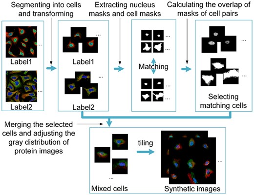
Flowchart of generating images of mixed patterns

2.2 Image representation by deep learning features

As the CNN model, bestfitting, has been demonstrated effective in protein image classification and its learned features have the ability to put multi-label proteins between clusters of single-location proteins (Ouyang et al., 2019), we used the bestfitting model to encode the subcellular location patterns in fluorescence images. The model was built by retraining DenseNet121 (Huang et al., 2017) using over 109 000 IF images from 28 subcellular location classes, with the loss function combining focal loss (Lin et al., 2017) and Lovász loss (Berman et al., 2018) to handle the class imbalance. To alleviate overfitting, data augmentation was utilized in the bestfitting during training and testing stage.

The input of the bestfitting model was 1024×1024 pixel IF images having protein channel and reference channels (nucleus, microtubules and ER). Because the images in the real dataset have no microtubules and ER channels, we set these two reference channels as background with gray values of 13, which was the average of those in HPA images. The output of bestfitting encoder were 1024-dimensional features from the penultimate layer and 28-dimensional features from the last layer, which were then used as image representations in pattern unmixing.

2.3 Pattern unmixing methods

In this work, it was assumed that a mixed pattern was an approximate linear combination of fundamental patterns, and also was influenced by variation of cell morphology and fluorescent staining (Zhao et al., 2005). Based on the deep features of protein patterns, one linear and three nonlinear unmixing algorithms were used to quantify the protein locations. Here, we supposed that the fundamental patterns were known, as they could be constructed by averaging image representations of single-location proteins. All of the unmixing algorithms utilized the fundamental patterns for solving the fractions.

2.3.1 Linear unmixing

Under the linear assumption, a mixed pattern can be expressed as products of a coefficient vector $\mathit{\alpha }\mathbf{=}\left[{\alpha }_1,{\alpha }_2,\mathrm{\dots .},{\alpha }_U\right]$ and fundamental patterns:

$$\left\{\begin{array}{l}\mathit{x}=\sum _{p=1}^U{\alpha }_p{\mathit{f}}_p+\mathit{e}\\ {\Vert \mathit{\alpha }\Vert }_1=1,\mathit{\alpha }\ge 0\end{array}\right.$$

(1)

where $\mathit{x}\in {\mathbb{R}}^{K\times 1}$ represents an image encoded by the bestfitting model (K represents the number of features), ${\mathit{f}}_p$ (p = 1, 2, …, U) represents the fundamental pattern of the pth subcellular location, ${\alpha }_p$ represents the proportion of pattern ${\mathit{f}}_p$ in the composition of the mixture, U is defined as the total number of fundamental patterns in the mixture, and $\mathit{e}$ is the error term that releases the difference between the true value $\mathit{x}$ and predicted value. The task of the problem is to calculate the mixture coefficient vector $\mathit{\alpha }$ by minimizing the error term ${\Vert \mathit{e}\Vert }_2^2$ under the constraint ${\displaystyle \sum _{p=1}^U}{\alpha }_p=1$ and non-negative constrain $\forall {\alpha }_p\ge 0$⁠.

2.3.2 R-NNMF nonlinear model

Robust-Non-negative matrix factorization (R-NNMF) model is a nonlinear unmixing model which was originally used in hyperspectral unmixing application (Févotte and Dobigeon, 2015). Here we used it to solve the problem of subcellular location pattern unmixing. The R-NNMF model can be expressed as Equation 2:

$$\left\{\begin{array}{l}\mathit{x}\approx \sum _{p=1}^U{\alpha }_p{\mathit{f}}_p+\mathit{r}\\ {\Vert \mathit{\alpha }\Vert }_1=1,\mathit{\alpha }\ge 0\end{array}\right.$$

(2)

where r represents the nonlinear term of the models. Equation 2 can also be shown as a non-negative matrix factorization problem for all samples:

$$\left\{\begin{array}{l} \mathit{X}\approx \mathit{F}\mathit{A}+\mathit{R}\\ \mathit{F}\ge 0,\mathit{A}\ge 0,\mathit{R}\ge 0\end{array}\right.$$

(3)

where A =$\left[{\mathit{\alpha }}_1,{\mathit{\alpha }}_2,\dots ,{\mathit{\alpha }}_N\right]$ represents the set of mixed fractions (N represents the total number of samples), F =$\left[{\mathit{f}}_1,{\mathit{f}}_2,\dots ,{\mathit{f}}_U\right]$ represents a set of fundamental patterns, and R =$\left[{\mathit{r}}_1,{\mathit{r}}_2,\dots ,{\mathit{r}}_N\right]$ includes the nonlinear term of all the predicted samples. The optimization expression of the minimization problem can be denoted as Equation 4:

$${\mathit{A}}^{*},{\mathit{F}}^{*},{\mathit{R}}^{*}=\arg \underset{\mathit{A},\mathit{F},\mathit{R}}{\min }D(\mathit{X}|\mathit{FA}+\mathit{R})+\theta {\Vert \mathit{R}\Vert }_{2,1}$$

(4)

where $D(\mathit{X}|\mathit{FA}+\mathit{R})$ represents the β-divergence (Févotte and Idier, 2011) between X and FA+R, and the divergence is defined as Equation 5:

$$D(\mathit{X}|{\mathit{X}}^{*})=\sum _i\sum _j\left({\mathit{X}}_{ij}\hspace{0.17em}\text{log}\hspace{0.17em}\frac{{\mathit{X}}_{ij}}{{\mathit{X}}_{ij}^{*}}-{\mathit{X}}_{ij}+{\mathit{X}}_{ij}^{*}\right)$$

(5)

In addition, $\theta$ is a non-negative hyperparameter to adjust the weight between the divergence term and the sparse penalty term. Here, it was set as 0.08. The sparse term of the model, ${\Vert \mathit{R}\Vert }_{2,1}$⁠, was calculated by Equation 6:

$${\Vert \mathit{R}\Vert }_{2,1}=\sum _{i=1}^N{\Vert {\mathit{r}}_i\Vert }_2$$

(6)

To handle the minimization problem Equation 4 subject to the constraint of ${\alpha }_p$ summed up to one, we initialized ${\mathit{A}}^{*}$ and ${\mathit{R}}^{*}$ based on singular value decomposition (Boutsidis and Gallopoulos, 2008) and ${\mathit{F}}^{*}$ based on fundamental patterns, and then updated them with block coordinate descent strategy. The algorithm for updating ${\mathit{R}}^{*}$ and ${\mathit{F}}^{*}$ is majorization–minimization, and for ${\mathit{A}}^{*}$ is a heuristic scheme algorithm (Dobigeon and Févotte, 2013). After the optimization, we used the β-divergence and the fundamental patterns F to adjust the order of coefficients in ${\mathit{A}}^{*}$ to match with the labels.

2.3.3 Multilinear mixture unmixing model

An alternative nonlinear mixing model is multilinear mixture (MLM) model extending from bilinear model (Wei et al., 2017). The formula of multilinear mixing model can be simply expressed as Equation 7:

$$\left\{\begin{array}{l}\mathit{x}=(1-\lambda )\mathit{F}\mathit{\alpha }+\lambda \mathit{F}\mathit{\alpha }\circ \mathit{x}+\mathit{e}\\ {\Vert \mathit{\alpha }\Vert }_1=1,\mathit{\alpha }\ge 0\\ 0\le \lambda \le 1\end{array}\right.$$

(7)

where $\circ$ denotes the Hadamard product, and $\lambda$ is a specific parameter for each sample controlling the tradeoff between linearity and nonlinearity. The optimization problem of above formula can be expressed as Equation 8:

$${\mathit{A}}^{*},{\mathit{F}}^{*},{\mathit{l}}^{*}=\arg \underset{\mathit{A},\mathit{F},\mathit{l}}{\min }\sum _{i=1}^N{\Vert {\mathit{e}}_i\Vert }_2^2$$

(8)

The A, F and l represent the coefficient matrix, base matrix and nonlinear parameter vector composing of all the $\lambda$⁠, respectively. To solve the optimization problem, block coordinate descent strategy (Beck and Tetruashvili, 2013) with gradient projection algorithm is adopted to update A, F and l. In the initialization of the three parameters, the nonlinearity vector l was set as zero, A was set as a linear unmixing result, and F was initialized with fundamental patterns. The result of the optimization problem converged to a stationary value with the error range below 10⁻⁸.

2.3.4 K-nonlinear unmixing model

This model is a kernel-based method that maps data from the original input space into a high-dimensional feature space, and resolves the linear problem in the new space (Chen et al., 2013). The formula of the model can be represented as Equation 9:

$$\left\{\begin{array}{l}\mathit{x}=\Psi (\mathit{\alpha },\mathit{F})+\mathit{e}\\ {\Vert \mathit{\alpha }\Vert }_1=1,\mathit{\alpha }\ge 0\end{array}\right.$$

(9)

The $\Psi$ denotes a nonlinear function defining the relationship between fundamental patterns and the mixed pattern. To get the mixed coefficient$\mathrm{ }\mathit{\alpha }$⁠, the nonlinear function $\Psi$ was mapped into Hilbert space denoted by $\psi$ to transform the nonlinear problem into a linear problem. Thus, the minimizing function of Equation 9 is defined as Equation 10:

$${\psi }^{*}=\underset{{\psi }^{*}}{\arg \min }\frac{1}{2}{\Vert \psi \Vert }^2+\frac{1}{2\mu }{\Vert \mathit{e}\Vert }_2^2$$

(10)

where $\psi ={\psi }_{\mathit{lin}}+{\psi }_{\mathit{nlin}}$ with ${\psi }_{\mathit{lin}}({\mathit{b}}_j)={\mathit{\alpha }}^T{\mathit{b}}_j$ subject to $e_j=x_j-\psi ({\mathit{b}}_j)$⁠. $x_j$ is the element of x, ${\mathit{b}}_j$ represents the row vector of base matrix F, and the parameter μ is used to control the tradeoff between regularization and fitting.

The kernel trick mapping from $\Psi$ to $\psi$ utilizes a polynomial kernel, which is defined as Equation 11:

$$\kappa ({\mathit{b}}_i,{\mathit{b}}_j)={\kappa }_{\mathit{\text{lin}}}\mathit{+}{\kappa }_{\mathit{nlin}}={{\mathit{b}}_i}^T{\mathit{b}}_j+{\left({{\mathit{b}}_i}^T{\mathit{b}}_j\right)}^2$$

(11)

Then, Lagrange function associated with Equation 10 was constructed and single iteration gradient projection algorithm (Rosen, 1961) was conducted to solve the problem for the mixture coefficients.

3 Results

3.1 Comparison of object-based features and deep features on the real dataset

As mentioned before, the previous works about protein quantitative analysis, including the works of Murphy group and the VW-SVM model, used only the features of fluorescence objects for image representation. The object-based features mainly include morphological and spatial features of objects, frequencies of different types of objects in each image, and fluorescence intensity of objects (Yang et al., 2016). We first investigated whether the features extracted by the deep model, bestfitting, can achieve more accurate representation than the object-based features.

Here t-SNE (Maaten and Hinton, 2008) was used to visualize the object-based features and bestfitting features of images in the real dataset. As shown in Figure 3A, the two subcellular locations, i.e. mitochondria (deep red points) and lysosomes (deep blue points), can be clearly differentiated by the features from the three encoders, while multi-label samples are found between the clusters of them. With the increasing fraction of lysosomes and decreasing of mitochondria, the color of points changes from deep red to deep blue gradually. It seems that the feature points of mixtures from the deep learning model are more evenly distributed in the feature space than the object features, which reveals that the deep learning features might be a more effective quantitative descriptor for mixed patterns.

Fig. 3.

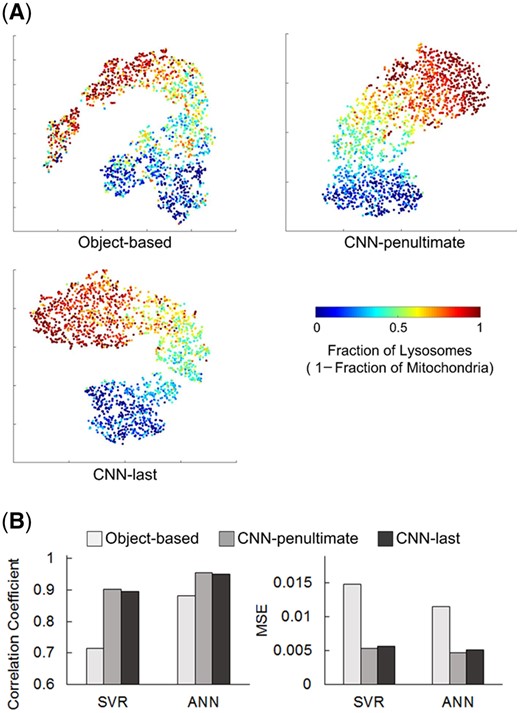
Comparison of the object-based features and deep features. (A) t-SNE visualization of object-based features and the bestfitting features from the penultimate layer and last layer, respectively. Each dot represents one image. (B) Regression results of using different feature sets on the real dataset

Then we fed each of the three feature sets into a support vector regression (SVR) (Smola and Schölkopf, 2004) and an artificial neural network (ANN) (Wang, 2003) model, respectively, and used 5-fold cross validation on the real dataset to assess the features. Correlation coefficients and mean-square errors (MSE) were calculated to represent the model performance (Fig. 3B). Detailed results on images with different fraction patterns were shown in Supplementary Figure S1. It can be seen that the deep learning features show better regression performance than the object features. This indicated that the features extracted by the bestfitting model contain more accurate and abundant subcellular localization information compared with the object-based features, which might help to improve quantitative analysis of subcellular location patterns. The regression results of the penultimate layer features had 0.9576 correlation coefficient with the ground truth, which was slightly higher than that of the last layer features.

Although the SVR and ANN models can achieve promising unmixing performance, they are supervised methods that need labeled data in the model construction. In fact, the subcellular locations of proteins are various and mostly have no quantitative annotations, so this study attempted to unmix the multi-label patterns without training supervised models.

3.2 Comparison of synthetic and real images

Synthetic dataset was constructed to enable more comprehensive evaluation of the unmixing methods (Table 1). The four subcellular location combinations in the synthetic dataset were selected through investigating the number of proteins belonging to each location, as well as the occurring frequency of multi-label patterns in the HPA database.

Table 1.

Details of the datasets used in this study

Dataset	Subcellular location combination	Number of images
Real dataset	Lysosomes and mitochondria	2056
Synthetic dataset	Cytosol and nucleoplasm	187
	Cytosol and plasma membrane	44
	Nucleoli and nucleoplasm	23
	Mitochondria and nucleoplasm	91

Figure 4 shows some examples of synthetic cells showing different protein fractions in cytosol and nucleoplasm, and example images of other three label combinations could be seen in Supplementary Figure S2. It can be seen that the protein (green) regions in the cells was visually similar with real cells labeled with cytosol and nucleoplasm in the HPA. Furthermore, we used t-SNE to visualize the real cells without quantitative annotation and the synthetic cells. Here, the real cells were derived from the images of U-2 OS cell line in the HPA, where they were annotated with cytosol and nucleoplasm subcellular location with enhanced or supported reliability score. Then, the real and synthetic cell images were padded and fed into the bestfitting model, and the penultimate layer features were used to conduct the visualization. It can be seen that the real and synthetic cells were mixed together, and the deep features can distinguish synthetic cells with different pattern fractions. This implied that our synthesis method can generate cell images very close to the real ones, and the synthetic images could be effectively used in test of unmixing methods.

Fig. 4.

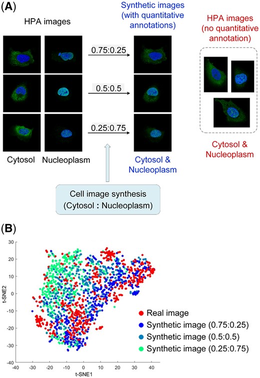
Comparison of synthetic and real cell images. (A) Examples of synthetic and real cells of the cytosol and nucleoplasm pattern. (B) t-SNE visualization

3.3 Performance of the unmixing methods

We compared the performance of the linear and nonlinear unmixing methods based on both the real dataset and the synthetic dataset. Each method was repeated ten times, and the mean correlation coefficients and ranges were shown in Figure 5, while MSEs and performance on different fraction patterns can be seen in Supplementary Figures S3 and S4. The K-nonlinear method achieved the best and most stable performance compared with other nonlinear methods, and had quite similar performance with the linear decomposition in this task. At the same time, we found that the linear unmixing method was prone to misclassify multi-label proteins as single locations, which means that the fractions of the dominant patterns are likely to be predicted as 1 and the other are predicted as 0. Specifically, among the multi-label images in the real dataset, over 10% are misclassified as single-label ones by the linear method, while the misclassification ratios of nonlinear methods are below 2% (Supplementary Table S1). Overall, the K-nonlinear method was more sensitive and accurate in detecting and unmixing the multi-label patterns.

Fig. 5.

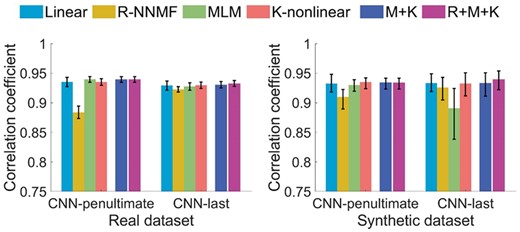
Results of different pattern unmixing methods. M + K represents the ensemble of MLM and K-nonlinear unmixing, and R + M+K represents the ensemble of all the three nonlinear unmixing methods

In addition, it can be observed that the features from the penultimate layer of the bestfitting network slightly outperformed these from the last layer. But in terms of the time spending on decomposing, the work using penultimate layer features was much more time-consuming (Supplementary Table S2). For example, the averaged computing time of K-nonlinear algorithm using the penultimate layer features was over one thousand times longer than that using the last layer features.

3.4 Construction of DULoc model

To build a final efficient solution of pattern unmixing, we combined the models by weighted sum of their results. Since all the three nonlinear algorithms have linear terms, we only integrated the nonlinear methods (Fig. 5). The weights were obtained by grid search. Twofold cross validation was performed on the real and synthetic dataset, respectively. Half of the data was used to grid search the best weight parameters, which were then used on the other half to get the unmixing results. The data partition was repeated for ten times, and the averaged correlation coefficients (Fig. 5) and MSEs (Supplementary Fig. S3) were shown. The ensemble models brought slightly improvements on the prediction. The learned weights on the K-nonlinear were much higher than those of other models, indicating that the K-nonlinear dominated the results. Besides, the ensemble models improved the stability and robustness of the prediction. The misclassification ratios of assigning the single label to multi-label images were decreased to 0 (Supplementary Table S1). In consideration of both accuracy and time spending, the final DULoc model were constructed by combining results of K-nonlinear with weight of 0.7556 and MLM with weight of 0.2444, and the features used in the decomposing were from the last layer of bestfitting model. Given an IF image of one protein and its qualitative subcellular locations, the built DULoc model could use constructed fundamental patterns to estimate fractions of the protein across the locations.

The DULoc was compared with a previous non-training pattern unmixing method proposed by Murphy group (Peng et al., 2010). On the real dataset, the predicted fractions of that model have 0.83 of correlation coefficient and 0.055 of MSE with the ground truth, while our DULoc can achieve over 0.93 of correlation coefficient and 0.017 of MSE. This indicated that using deep features and combining multiple unmixing algorithms can lead to a promising result in the quantitative subcellular location prediction.

3.5 Large-scale pattern unmixing for images in the HPA

To further validate the ability of our method in estimating protein amounts, we applied the DULoc on the IF images annotated with ‘main location(s)’ and ‘additional location(s)’ in the HPA database. The database marked each of the subcellular locations annotated to one protein as main or additional according to the protein staining intensity. For example, protein RPL9 was annotated as localized to endoplasmic reticulum, cytosol and nucleoli, in which the former two are main locations and the last is an additional location for this protein. These annotations allowed us to assess our model. Here, a subset of representative IF images of proteins from the HPA Cell Atlas (HPA v20) were used. These images were annotated with both main and additional locations, and the reliability scores of these annotations were enhanced or supported. The images were from three cell lines, i.e. U-2 OS, A-431 and U-251 MG, which have the most abundant images of stained proteins. To exclude the effect of single-cell level expression, the images with description of single-cell variations or cell cycle-dependent variations were removed. Thus, 2100 images having main and additional locations were employed as test samples in this application. When performing the DULoc unmixing, fundamental pattern representations were generated by deriving single-location proteins from the HPA and averaging the bestfitting features.

For one protein, it was assumed that its fraction(s) in main location(s) was/were higher than those in additional location(s). So, the image samples whose lowest fraction for main location(s) was higher than the highest fraction for additional location(s) were regarded as being predicted correctly. If only one of the locations was predicted as 1 and all the other locations was predicted as 0, it means that the sample was misclassified as single-locational, and the case would be regarded as a wrong prediction. The consistency between the model predictions and HPA annotation orders was defined as ratio of images that had correct predictions.

It is noted that our method can handle with images having over two subcellular locations. Table 2 lists the consistency results of applying DULoc and linear method on the test images of the three cell lines. Both of the methods used the bestfitting last layer features. The results showed performance of the DULoc was better than the linear unmixing, as the overall consistencies of DULoc results for U-2 OS, A-431 and U-251 MG were 71.87%, 72.20% and 64.93%, respectively, while the results of linear method were 63.64%, 65.56% and 59.73%, respectively. What is more, it is the same trend for all the cell lines that the more locations the model unmixing, the lower consistency it shows. This assessment by using the annotations in the HPA can be considered as a reference to prove the predictive ability of our model.

Table 2.

Comparison of the performance between the linear unmixing method and DULoc in the large-scale prediction for the HPA images

Cell line	Number of labels	Number of images	Ratio of correct predictions (linear method)	Ratio of correct predictions (DULoc method)
U-2 OS	Double	632	71.68%	81.96%
	Triple	271	49.08%	52.40%
	Quadruple	32	28.13%	37.50%
A-431	Double	471	71.97%	81.32%
	Triple	227	56.83%	58.15%
	Quadruple	25	24.00%	28.00%
U-251 MG	Double	275	65.46%	72.73%
	Triple	153	51.63%	52.94%
	Quadruple	14	35.71%	42.86%
In total		2100	63.48%	70.52%

In addition, we also investigated the performance of DULoc when using the features of the penultimate layer as image representations (Supplementary Table S3). The ratio of correctly predicted images was 69.05%, slightly lower than the DULoc using last layer features. This indicated that using the last layer features could achieve good results with low time cost in the large-scale validation experiment.

4 Conclusions

In this study, we proposed a DULoc for quantitative analysis of multiplex protein subcellular localizing patterns. The DULoc model used a pre-trained convolutional neural network to extract protein patterns, and combined two nonlinear methods for pattern unmixing. Given an IF image with known subcellular locations, the model can estimate the fractions of the protein in these locations. The performance of DULoc achieved 0.93 of correlation coefficient on the real dataset, which outperformed existing models. Moreover, on the synthetic dataset having multiple patterns of subcellular location combinations, this model can also achieve high correlation coefficient with ground truth. Besides, the application of DULoc on the large-scale quantitative prediction of images in the HPA database demonstrated that our approach can achieve better performance than the linear unmixing, indicating its utility in practice.

In future works, we intend to further enhance the accuracy and robustness of the unmixing model, especially the performance on complex subcellular location patterns. In addition, for increasing the image data with reliable quantitative annotations, deep generative models would be applied to create IF cell images with exact quantitative labels. Finally, current protein locations are assigned for all cells together in one image, but there exists single-cell heterogeneity in subcellular pattern, so developing models capable of segmenting and labeling each individual cell with precise quantitative subcellular distribution would be an important direction.

Funding

This work was supported in part by the National Natural Science Foundation of China [61803196], the Natural Science Foundation of Guangdong Province of China [2018030310282] and the Science and Technology Program of Guangzhou [202102021087].

Conflict of Interest: none declared.