


Abstract
Motivation: The systematic study of subcellular location pattern is very important for fully characterizing the human proteome. Nowadays, with the great advances in automated microscopic imaging, accurate bioimage-based classification methods to predict protein subcellular locations are highly desired. All existing models were constructed on the independent parallel hypothesis, where the cellular component classes are positioned independently in a multi-class classification engine. The important structural information of cellular compartments is missed. To deal with this problem for developing more accurate models, we proposed a novel cell structure-driven classifier construction approach (SC-PSorter) by employing the prior biological structural information in the learning model. Specifically, the structural relationship among the cellular components is reflected by a new codeword matrix under the error correcting output coding framework. Then, we construct multiple SC-PSorter-based classifiers corresponding to the columns of the error correcting output coding codeword matrix using a multi-kernel support vector machine classification approach. Finally, we perform the classifier ensemble by combining those multiple SC-PSorter-based classifiers via majority voting.
Results: We evaluate our method on a collection of 1636 immunohistochemistry images from the Human Protein Atlas database. The experimental results show that our method achieves an overall accuracy of 89.0%, which is 6.4% higher than the state-of-the-art method.
Availability and implementation: The dataset and code can be downloaded from https://github.com/shaoweinuaa/.
Contact: dqzhang@nuaa.edu.cn
Supplementary information: Supplementary data are available at Bioinformatics online.
1 Introduction
One important task in the research of proteomics is to explore the natural function of proteins in performing and regulating the activities of an organism at cell level (Breker and Schuldiner, 2014). It is widely recognized that the function of a protein is closely associated with its corresponding cellular compartments (Chebira et al., 2007). Proteins can only find their correct interacting molecules at the right place. Thus, subcellular location can provide important clues for understanding the function of a protein. With the breakthrough of genome sequencing and bioimaging techniques, traditional time-consuming and expensive wet-laboratory experimental approaches cannot catch up with the speed of newly known proteins (Zhang et al., 2006). Hence, finding an automatic computational way to determine the subcellular locations of proteins has been becoming a focus in computational biology (Glory and Murphy, 2007). From the perspective of machine learning, this task can be transformed into a multi-class or multi-label classification problem. This is a two-step framework, where we first need to figure out a proper feature representation way for encoding the protein data, which then will be fed into a trained machine learning model for label decision. There are two major research categories depending on how the protein data are represented, i.e. one-dimensional amino sequence and two-dimensional image (Xu et al., 2013).
On one hand, if a protein is represented in amino acid sequence, PseAAC (Chou, 2001), PSSM (Jeong et al., 2011; Pierleoni et al., 2011) and gene ontology (Chi, 2010) are among the applied sequence-based features. In the second step, various machine learning algorithms have been proposed. For instance, researchers in Yoon and Lee (2012) adopted a boosting framework to accomplish the classification task, and in Wang and Li (2013), a random label selection method was presented to learn the label correlations from training dataset to guide the classification for multi-label proteins.
On the other hand, accompanied with the explosive increments in genomic data, we witnessed great advances in automated microscopic imaging in recent years (Peng et al., 2012). Because of the intuitive characteristics of images compared with amino acid sequence, bioimage-based protein subcellular distribution pattern analysis has attracted much attention. For example, it is found that image-based analysis can be successfully used to detect protein biomarkers, which will dynamically change their subcellular locations in the cancerous tissues (Kumar et al., 2014; Xu et al., 2013, 2015).
If proteins are represented with two-dimensional images, e.g. through fluorescent or immunohistochemistry microscopy, the most widely used image features can be grouped into two categories, i.e. global and local features. For global feature, the DNA feature (Boland and Murphy, 2001) is designed to characterize DNA distribution in a cell image. Since there is high co-occurrence of protein and DNA in a protein image, we can infer the relative position of protein according to the DNA distribution. Besides, Haralick feature based on db wavelet is another global feature to describe image texture such as inertia and isotropy, which is demonstrated to be robust to cell rotations and translations (Murphy et al., 2003; Newberg and Murphy, 2008). As to local feature, LBP (Ojala et al., 1996) feature is the most frequently applied descriptor to characterize the spatial structure of images involving flat areas, edges and spots. Some extensions are also reported. Yang et al. (2014) constructed a mixed local feature set by adding two extensive forms of LBP, i.e. LTP (Tan and Triggs, 2010) and LQP (Nanni et al., 2010). Coelho et al. (Coelho et al., 2013) applied the SURF feature to handle the classification problem in cell images.
Considering different features will have their own advantages, a common strategy is to fuse multiple types of features. For instance, different features are concatenated as a long vector to perform the subsequent classification task (Newberg and Murphy, 2008; Xu et al., 2013; Yang et al., 2014). Intuitively, since single type of features cannot reflect all the information of a protein image, fusing multiple types of features together is expected to be a more promising way.
For learning algorithms design, Boland et al. (1998) applied neural networks to classify four protein types; Yang et al. (2014) proposed a probability-based support vector machine (SVM) to predict the subcellular location of proteins in human reproductive system. By considering a high ratio of human proteins co-exist at different locations, Xu et al. (2013) designed a multi-label classification classifier. Other efforts include Chebira et al. (2007) used a multi-resolution approach, and logistic regression algorithm with latent variables was proposed in Li et al. (2012).
Although much progress has been achieved in designing different statistical classifiers, to the best of our knowledge, none of the existing image-based classifiers takes the biological cell structure information into consideration, which has already been demonstrated to be effective in solving biological sorting problems (Lin et al., 2011). The basic hypothesis of existing predictors is to parallelly consider every cellular component class regardless of their organizations in the cell. It is expected that better performance will be achieved when we incorporate the cell nature component organization structure into the model construction.
To enable the learned model to incorporate the subcellular component organization structure, we propose a new classifier learning approach by utilizing the error correcting output coding (ECOC) framework (Dietterich and Bakiri, 1995). This new approach can decompose the multi-class problem into several binary classification problems according to the prior human cell structural information. The final decision will then be made by combining the results of these binary classifiers. In the new structure-driven learning approach, we first construct a codeword matrix to reflect the biological structure of cellular compartments with ECOC. Then, for each binary classifier corresponding to the columns of the ECOC codeword matrix, we use kernel combination method to fuse different types of features rather than the direct combination strategy. Finally, we perform the classifier ensemble by combining multiple classifiers via majority voting. The experimental results show that our method performs much better than several state-of-the-art methods, because the proposed approach has incorporated the cell structure prior knowledge into model generation.
2 Materials and methods
2.1 Dataset
Starting from 2005, the researchers use the antibody-based technique to functional study of the human proteome and build the well-known Human Protein Atlas (HPA) database (Uhlen et al., 2005). In the recent 13th version of HPA database, 86% of human genome is involved. Specifically, 16 ;975 genes with 24 028 antibodies have been covered to 46 different normal human tissues and 20 different cancer types.
In this study, we have generated a collection of 1636 immunohistochemistry images with high validation and objective scores (Ponten et al., 2008) from HPA as our benchmark dataset. It contains 21 proteins related to 46 normal human tissues. And each image belongs to one of the seven most frequently appeared subcellular locations, namely, cytoplasm, Golgi apparatus, mitochondrion, vesicles, nucleus, endoplasmic reticulum and lysosome. Table 1 summarizes the distribution of our dataset.
The distribution of the benchmark dataset
| Category | Size |
|---|---|
| Cytoplasm | 391 |
| Golgi apparatus | 228 |
| Mitochondrion | 319 |
| Vesicles | 139 |
| Nucleus | 183 |
| Endoplasmic reticulum | 216 |
| Lysosome | 160 |
| Total | 1636 |
| Category | Size |
|---|---|
| Cytoplasm | 391 |
| Golgi apparatus | 228 |
| Mitochondrion | 319 |
| Vesicles | 139 |
| Nucleus | 183 |
| Endoplasmic reticulum | 216 |
| Lysosome | 160 |
| Total | 1636 |
2.2 Overview of our method
Figure 1 shows the flowchart of our method, which consists of four major steps. First, we extract and select features from the given protein images. Then, we use ECOC method to transform the multi-class classification problem into a series of binary classification sub-problems according to a pre-defined codeword matrix. Here, the codeword matrix comprised 14 bits. The first six bits are designed according to the biological structure of cellular compartments, which can bring more prior information to the learning process. And the other eight checking bits are used to strengthen the error-correcting ability of this ECOC-based model. Next, since db wavelet was employed to get the multi-resolution global feature (i.e. Haralick feature), we can construct 10 different SC-PSorter models based on different sets of features extracted from 10 vanishing moments of db wavelets. Moreover, for each SC-PSorter model, we construct 14 multi-kernel-based SVM classifiers corresponding to the columns of the ECOC codeword matrix. Finally, we perform the classifier ensemble by combining those 10 SC-PSorter-based classifiers via majority voting.
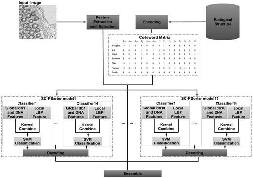
The flowchart of our proposed method
2.3 Feature extraction and selection
For protein images, different types of features (i.e. global and local features) are expected to provide complementary information (Yang et al., 2014). Therefore, we are encouraged to use both of the two types of features to describe protein images. Specifically, as to global feature, we select Haralick feature with 10 different vanishing moments from 1 to 10, then for each vanishing moment, an 836-dimensional feature can be obtained. In addition, a four-dimensional global DNA feature is also incorporated due to their values in inferring the relative position of protein. As to local feature, we prefer to choose the most widely used LBP feature, which is constituted by a 256-dimensional vector. Hence, for every protein image, we can get a 1096-dimensional descriptor for each db wavelet if we directly combine them together. After that, to reduce computational time cost and avoid overfitting, we select the most distinguishing features by applying the stepwise discriminant analysis method (Huang et al., 2003).
2.4 Error correcting output coding
In this article, our goal is to determine the subcellular location that a protein image belongs to. Since there are seven subcellular locations, this problem can be regarded as a multi-class classification problem. Nowadays, multi-class classification is an important issue in many machine learning domains, such as text classification (Nigam et al., 2000), and medical analysis (Lu et al., 2005). There are two main lines to deal with such multi-class learning problems, including ‘direct multi-class representation’ and ‘(indirect) decomposition design’. The first line aims to design multi-class classifiers directly, such as neural network (Boland et al., 1998) and multi-class SVMs (Yang et al., 2014). In contrast, the second line endeavors to first transform the original multi-class problem into several binary classification problems and then to combine the results of these binary classifiers for making final decision. As a typical indirect decomposition way to deal with multi-class problems, ECOC (Dietterich and Bakiri, 1995; Liu et al., 2015, b) is one of the representative methods. Specifically, there are three main steps in ECOC-based classification system, including (i) encoding, which decomposes the original problem into several binary classification problems; (ii) binary classifier learning and (iii) decoding, which makes a final decision based on the outputs of those binary classifiers. In the following, we will introduce each step in detail.
2.4.1 Encoding
In the encoding procedure, a codeword matrix is employed to decompose the original multi-class problem into several binary sub-problems. Here, the rth row of (i.e.) represents the codeword of the rth class, while each column of denotes the new class label vector for each of original classes. The elements in each column of the codeword matrix can be set as −1, 0, and 1 in ternary ECOC encoding methods and −1 and −1 in binary ECOC encoding methods (Pujol et al., 2006). Below, we briefly introduce two typical ECOC encoding strategies including one-versus-all coding and the forest coding (Escalera et al., 2007).
1) One-versus-all coding
2) Forest coding
In this data-dependent coding strategy, the codeword matrix is completely determined by the partition of the dataset by using the decision tree algorithm. Here, when building decision tree, each node corresponds to the best bi-partition of the set of classes by maximizing the mutual information between different types of samples. The process is recursively applied until sets of single classes corresponding to the tree leaves are obtained.
2.4.2 Binary classifier learning
The second step is to train multiple binary classifiers based on the codeword matrix. Specifically, a binary classifier is corresponding to a specific column of the codeword matrix, where the samples labeled as 1 are used as positive instances, and samples labeled as −1 are regarded as negative instances. It is worth noting that those instances labeled as 0 will not be used for training the classifier in ternary encoding methods. Given a codeword matrix that contains l columns, we then learn a total of l binary classifiers. In the literature, these binary classifiers are usually directly taken from many existing classifiers (e.g. SVM) (Escalera et al., 2007).
2.4.3 Decoding
2.5 ECOC coding with biological structural information
As mentioned in Section 2.4, ECOC-based methods transform the multi-class classification problem into a series of binary classification sub-problems according to a pre-defined codeword matrix. Different designs of codeword matrix may lead to different partitions of original classes, which will affect the classification performance. Hence, the design of the codeword matrix is important for ECOC-based methods. On the other hand, it is highly recognized that the biological structural information (Lin et al., 2011) plays a crucial role in determining protein subcellular location. Intuitively, such structural information can be used to guide the codeword matrix design, which can bring more prior information to the learning process and boost the learning performance. Accordingly, we design a codeword matrix according to the hierarchical structure of cellular compartments. In Table 2, we illustrate the proposed codeword matrix by taking advantage of the cellular compartments structure shown in Figure 2.
Corresponding coding matrix to the biological structure of cellular compartments
| Location | h root | h intra | h cyto | h sp | h meta | h modi |
|---|---|---|---|---|---|---|
| Cytoplasm | −1 | 1 | 1 | 0 | 0 | 0 |
| ER | 1 | 0 | 0 | −1 | 0 | 1 |
| Golgi | 1 | 0 | 0 | −1 | 0 | −1 |
| Lysosome | 1 | 0 | 0 | 1 | 1 | 0 |
| Mitochondrion | −1 | 1 | −1 | 0 | 0 | 0 |
| Nuclear | −1 | −1 | 0 | 0 | 0 | 0 |
| Vesicle | 1 | 0 | 0 | 1 | −1 | 0 |
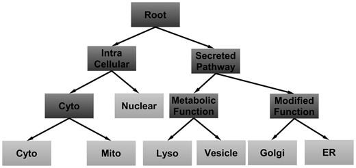
Biological structure of cellular compartments
As listed in Table 2, we derive six binary classifiers from this codeword matrix. Starting from roots, we use classifier hroot to distinguish between three intra-cellular compartments and the other four secreted pathway-based compartments. Then, for the splits under inter-cellular compartments, we apply hintra to discriminate nuclear and cytoplasm internal node, a union of proteins in cytoplasm and mitochondrion. Similar to hintra, hcyto is another classifier that is applied to characterize the differences between cytoplasm and mitochondrion. Pointing to the right sub-tree of root node, since the main function of vesicle is to uptake and transport of materials within the cytoplasm, and lysosome is capable of breaking down all kinds of biomolecules, they can be categorized into metabolic functional compartments. Moreover, the main functions of Golgi apparatus and ER are modifying the proteins for cell secretion, so classifier hsp is applied to distinguish the cellular compartments having either metabolic or modified functions under the node of secreted pathway. Finally, hmeta and hmodi are also constructed to classify the compartments within the nodes of metabolic function and modified function shown in Figure 2. In this work, we will mainly use this coding pattern to predict protein subcellular location under ECOC framework. Moreover, in the work by Lin et al. (2011), they also utilize the biological structure information and then build a tree-based classifier to predict the sequence-based protein subcellular location. Here, we will compare our proposed ECOC-based method with the method by Lin et al. in Supplementary Section S5 in the Supplementary Material.
2.6 ECOC coding by adding checking bits
From the detailed analysis in Supplementary Section S4, it is worth noting that, although the codeword matrix shown in Table 2 follows the biological structure shown in Figure 2, it has no error-correcting ability for the HDs between pairs of codewords are too short (e.g. there is only 1 bit difference between the codewords under the nodes of cytoplasm, metabolic function and metabolic function). So, to strengthen the error-correcting ability of the codeword matrix shown in Table 2, we add eight checking bits for each codeword of cellular compartment (shown in Table 3) to enlarge the HDs between pairs of codewords.
The added eight checking bits to enlarge the HDs between pairs of codewords
| Location | c 1 | c 2 | c 3 | c 4 | c 5 | c 6 | c 7 | c 8 |
|---|---|---|---|---|---|---|---|---|
| Cytoplam | 1 | 1 | 0 | 0 | 1 | 0 | 0 | 0 |
| ER | −1 | 0 | 1 | 0 | 0 | 0 | 1 | 0 |
| Golgi | −1 | 0 | 1 | 0 | 0 | 0 | 0 | 1 |
| Lysosome | 0 | −1 | 0 | 1 | 0 | 0 | −1 | 0 |
| Mitochondrion | 1 | 1 | 0 | 0 | 0 | 1 | 0 | 0 |
| Nuclear | 0 | 0 | −1 | −1 | −1 | −1 | 0 | 0 |
| Vesicle | 0 | −1 | 0 | 1 | 0 | 0 | 0 | −1 |
As listed in Table 3, the newly added eight checking bits are used for distinguishing different nodes or cellular compartments (e.g. c1 is used to distinguish between modified function and cytoplasm-based proteins), which cannot reflect the hierarchical structure of cellular compartments in Figure 2. So, after adding these eight checking bits, each cellular compartment is represented by 14 bits and the HDs between pairs of codewords are accordingly enlarged (e.g. the HD between the codewords under the nodes of Cytoplasm is enlarged from 2 to 4 if we add the eight checking bits).
2.7 Kernel combination
As the second procedure in ECOC framework, binary classifier learning is also important for multi-class classification. To better make use of different kinds of features, we adopt a kernel combination method (Wang et al., 2008; Zhang et al., 2011) to design each of multiple binary classifiers in ECOC. Specifically, for each dichotomy, we fuse both the global features (i.e. Haralick feature and DNA feature) and the local features (i.e. LBP) by a multi-kernel-based SVM classifier (Wang et al., 2008; Zhang et al., 2011).
2.8 Ensemble classification method
As can be observed from Figure 1, db wavelet has 10 vanishing moments from db1 to db10. Accordingly, we construct 10 SC-PSorter-based classification models, with each one corresponding to a specific type of vanishing moments. Inspired by Liu et al. (2015a), Xu et al. (2013) and Yang et al. (2014), we adopt a majority voting strategy to combine those SC-PSorter-based models together. Specifically, for a testing protein image , if the ith (I = 1, 2, , 10) SC-PSorter model predicts that it belongs to the location , the vote for the cth compartment is added by one. Then, is in the location with the largest vote-based on all of the 10 SC-PSorter models.
3 Experimental results
3.1 Experimental settings
In previous works (i.e. Xu et al., 2013; Yang et al., 2014), researchers use images from the same protein for training and testing via cross-validation. Following these works, in our experiment, we use the same cross-validating strategy. Specifically, we equally divide the images in each protein into five disjoint subsets, with four subsets used for training and the remaining subset used for testing. For all the proposing and comparing methods in this article, the SVM classifier is implemented by using LIBSVM toolbox (Chang and Lin, 2011), with an RBF kernel and the parameter is tuned from 0.9 to 2.1 at a step size of 0.1 by using grid search on the training data. Also, for each feature in the training set, a common feature normalization scheme is adopted, i.e. the normalized feature , where is the maximum value of the ith feature in the training set. Also, the value will be used to normalize its corresponding feature in the test set.
3.2 Results for combining different types of features
To evaluate the efficacy of using different types of features, we first perform experiments by only using one type of features(i.e. the global feature and local feature) and combining different types of features together (i.e. direct combine and kernel combine) to predict the targets of proteins. Here, we choose the one-versus-all coding strategy, with experimental results shown in Figure 3. As can be seen from Figure 3, on one hand, direct combination of different types of features will not lead to the improvements of prediction accuracies. In most cases, the classification accuracies for this combination strategy are between using global or local feature only. On the other hand, using kernel combination method to fuse different types of features is a much more effective way, where classification accuracies consistently outperform those methods based on one single type of features (i.e. global feature or local feature). However, even for the kernel combination strategy, the classification accuracies cannot achieve to 70% for all of the 10 db wavelets, which reminds us to replace the simple one-versus-all coding strategy with other coding strategies for further improving.
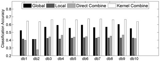
Classification accuracies by using single type of features and combining different types of features together
3.3 Results for different coding strategies
In the second groups of experiments, we test the classification performances for three different coding strategies, namely, one-versus-all, forest and biological structural-based coding strategies (i.e. following the codeword matrix shown in Table 2), which are denoted as OVA-PSorter, F-PSorter and S-PSorter, respectively. Here, we also use kernel combination method to fuse global features (including both Haralick features and DNA features) and local features (i.e. LBP features) due to its superior classification performances in the first group of experiments. Figure 4 shows the classification accuracies by using all of the 10 db wavelets.
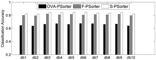
Performance comparison among different coding strategies
As can be seen from Figure 4, our proposed S-PSorter method consistently outperforms the other two methods (i.e. OVA-PSorter and F-PSorter), which shows the advantage of using the biological structure of cellular compartments to design the codeword matrix. On the other hand, Figure 4 indicates that F-PSorter achieves consistently better classification accuracies than OVA-PSorter. This is because F-PSorter constructs codeword matrix by maximizing the mutual information between different classes rather than the simple one-versus-all coding strategy used in OVA-PSorter. Moreover, we also compare the computational efficiency of different coding strategies in Supplementary Section S8.
3.4 Further improvement by adding checking bits
As discussed in Section 2.6, we also add eight checking bits (shown in Table 3) to the codeword matrix of S-PSorter model to strengthen its error-correcting ability. Here, we denote two ECOC-based methods, whose codeword matrices are derived by adding these eight checking bits to the S-PSorter-based codeword matrix and only using these eight checking bits, as SC-PSorter and C-PSorter, respectively. Figure 5 presents the individual classification accuracies of the above two methods when comparing with S-PSorter method for all of the 10 db models.
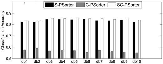
Performance comparisons among S-PSorter, C-PSorter and SC-PSorter methods
As can be seen from Figure 5, on one hand, SC-PSorter consistently outperforms S-PSorter on all of the 10 db wavelets. This is because we enlarge the HDs between pairs of codewords, and thus a few mistakes in some bits can be corrected by the decoding procedure. On the other hand, Figure 5 also shows the classification accuracies of C-PSorter method are consistently inferior to the other methods, which is because these eight checking bits are just designed to distinguish different nodes or cellular compartments, and they do not reflect the hierarchical structure of cellular compartments shown in Figure 2. (Detailed classification results are reported in Supplementary Section S4.)
3.5 Ensemble results with different coding strategies
As shown in Figures 4 and 5, for each method (i.e. OVA-PSorter, F-PSorter, S-PSorter and SC-PSorter), the classification accuracies from its individual 10 classifiers are different, which motivates us to utilize an ensemble strategy for better fusing the complementary individual decisions. Here, we use the majority voting strategy introduced in Section 2.8 to combine different classifiers together. Table 4 compares the classification accuracies of the best individual classifier and the ensemble model for these 4 methods (i.e. OVA-PSorter, F-PSorter, S-PSorter and SC-PSorter)
Comparison between individual and ensemble classification for four different coding strategies
| Method | Best independent classifier | Ensemble prediction |
|---|---|---|
| OVA-PSorter | 0.675 | 0.679 |
| F-PSorter | 0.819 | 0.853 |
| S-PSorter | 0.848 | 0.874 |
| SC-PSorter | 0.860 | 0.890 |
| Method | Best independent classifier | Ensemble prediction |
|---|---|---|
| OVA-PSorter | 0.675 | 0.679 |
| F-PSorter | 0.819 | 0.853 |
| S-PSorter | 0.848 | 0.874 |
| SC-PSorter | 0.860 | 0.890 |
As listed in Table 4, we can always obtain better classification accuracies when performing the classifier ensemble via majority voting. Table 4 also indicates that the classification accuracy of our proposed SC-PSorter method is improved from the best individual classifier of 0.860–0.890, which is the best overall classification accuracy among all of the four methods.
4 Discussion
4.1 Comparisons with existing works
We also compare our SC-PSorter method with several existing approaches for image-based prediction of protein subcellular location. For example, in Xu et al. (2013), the authors construct k SVM models where k is the number of classes. In training the ith SVM model, examples belonging to the ith class are seen as positive samples, while the other examples as negative samples. For a query protein image , the output vector consists of k probabilities related to k different subcellular locations. We say belongs to the class with the largest probability in the output vector. Different from Xu et al. (2013), the authors in Yang et al. (2014) construct k(k − 1)/2 SVM classifiers where each one is trained from two different classes. Then, the testing sample is fed into these k(k − 1)/2 SVMs and these classifiers also output a probability denoting which class it belongs to. Here, the SVM classifier is implemented with RBF kernel and the parameter is also tuned from 0.9 to 2.1 at a step size of 0.1 by using grid search on the training data.
Figure 6 presents the individual classification accuracies of the above two methods when comparing with our proposed SC-PSorter method. As can be seen from Figure 6, our proposed SC-PSorter method consistently achieves better classification accuracies than the other two approaches. Here, the better classification accuracies of our method are mainly owing to the following two aspects: (i) since the prior biological information is crucial in computational biology, we use the biological structural information to guide the learning procedure and (ii) we apply the multiple kernel combination strategy to fuse different types of features, which is regarded as a much more effective and flexible way than the direct combination strategy applied in the other two methods.
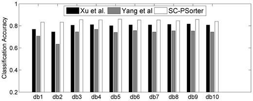
Classification accuracies achieved by SC-PSorter and the other two methods
We also compare the classification accuracies of the best individual classifier and the ensemble model for the above three methods. As listed in Table 5, for these three methods, we obtain better classification accuracies when performing the classifier ensemble via majority voting than the best individual classifier. On the other hand, Table 5 also indicates that, by performing the ensemble strategy, the SC-Porter method achieves the best classification accuracy among all of the three methods. This result again validates the advantage of our proposed SC-PSorter method for prediction of protein subcellular location.
Comparison between individual and ensemble classification for three different methods
| Method | Best independent classifier | Ensemble prediction |
|---|---|---|
| Xu et al . | 0.817 | 0.826 |
| Yang et al . | 0.768 | 0.772 |
| SC-PSorter | 0.860 | 0.890 |
| Method | Best independent classifier | Ensemble prediction |
|---|---|---|
| Xu et al . | 0.817 | 0.826 |
| Yang et al . | 0.768 | 0.772 |
| SC-PSorter | 0.860 | 0.890 |
4.2 Diversity analysis
For the purpose of understanding how our proposed ensemble SC-PSorter works, we endeavor to apply the kappa measure (Rodriguez and Kuncheva, 2006) to plot the diversity-error diagram, which evaluates the level of agreement between the outputs of two individual classifiers. In Figure 7, we show the diversity-error diagrams of ensemble SC-PSorter and the methods in Xu et al. (2013) and Yang et al. (2014) for the task of predicting protein subcellular locations. In our experiment, each ensemble contains 10 individual classifiers, with each corresponding to a specific classifier using different global db features. The value on the x-axis of a diversity-error diagram denotes the kappa diversity of a pair of classifiers in the ensemble, while the value on the y-axis is the averaged individual error of a pair of classifiers. Since a small value of kappa diversity indicates better diversity and a small value of averaged individual error indicates a better accuracy, the most desirable pairs of classifiers will be close to the bottom left corner of the graph. As shown in Figure 7, our proposed ensemble SC-PSorter achieves much lower kappa value and much lower classification errors than the methods in Xu et al. (2013). At the same time, our proposed SC-PSorter method is not as diverse as the method in Yang et al. (2014), but apparently, it has more accurate base classifiers than the method in Yang et al. (2014). It seems that our proposed method can achieve a better trade-off between accuracy and diversity than the compared two methods. That is, it builds a classifier ensemble based on the reasonable diverse but markedly accurate individual components.
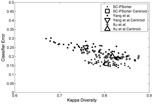
The diversity-error diagrams of classifiers in the task of determining protein subcellular locations
4.3 Slight variations on tree structure
We design another two variants of the hierarchy of cellular compartments (i.e. T1 and T2 are shown in Supplementary Figs. S1 and Supplementary Data in Supplementary Section S1, respectively), which are constructed by making slight variations on the tree structure in Figure 2. Specifically, on one hand, for the tree representation T1, we neglect the hierarchical structure of four cellular compartments (i.e. lysosome, vesicle, Golgi and ER) under the node of secreted pathway. On the other hand, for the tree representation T2, we misuse cytoplasm (which is originally under the node of intra cellular) as a metabolic functional compartment (under the node of secreted pathway).
The classification results in Supplementary Table S3 in the Supplementary Section S1 shows that the slight variations on the tree structure in Figure 2 will lead to decreases in the classification accuracies for all of the 10 db models when comparing with S-PSorter method. Also, as can be seen from Supplementary Table S4 in the Supplementary Section S1, the ensemble classification results for these two tree representations (i.e. T1 and T2) are 0.866 and 0.842, respectively, which are still higher than those of previously published methods (i.e. Xu et al. 2013; Yang et al. 2014), although a bit lower than our original S-PSorter method. These results suggest that the proposed tree representation in Figure 2 reflects the true hierarchy of subcellular compartments.
4.4 Prediction on unseen proteins
As mentioned in Section 3.1, we use images from the same protein to evaluate the performance of SC-PSorter method. However, a strict test, i.e. recognizing subcellular patterns in new protein, is also very important. So we have added one more experiment to compare SC-PSorter method with the other two methods (i.e. Xu et al. 2013; Yang et al. 2014) for predicting proteins that are not included in the training set (detailed in Supplementary Section S3).
As can be seen in Supplementary Table S6, our proposed SC-PSorter method consistently achieves better classification accuracies than the other two approaches for all of the 10 db wavelets. Moreover, when performing the classifier ensemble via majority voting, the classification accuracies for SC-PSorter, Xu et al. (2013) and Yang et al. (2014) methods are 0.809, 0.684 and 0.603, respectively. This result again validates the advantage of our proposed SC-PSorter method for the prediction of protein subcellular location.
5 Conclusion
In this article, we develop and test a novel prediction model, SC-PSorter, for determining image-based protein subcellular locations. Specifically, we first devise a novel codeword matrix by considering the biological structural information under the ECOC framework, and then for each binary classifier corresponding to the columns of the ECOC codeword matrix, we adopt kernel combination method to fuse different types of features. Finally, we develop a classifier ensemble by combining multiple SC-PSorter-based classifiers via majority voting.
In this study, our method has been shown effective in case of each protein corresponding to only one location. However, as a matter of fact, nearly 20% percentage of human proteins co-exist more than two locations (Zhu et al., 2009), and thus we will design a new method to solve this multi-label-based protein classification problem. Also, since different biomarker may provide complementary information for the prediction of protein subcellular location (Breker and Schuldiner, 2014), we will add non-image data (e.g. amino acid sequence) to our image-based predictor for further performance improvement.
Acknowledgements
We thank Prof. Hongbin Shen for his helpful suggestions and the anonymous reviewers for valuable comments.
Funding
This work was supported in part by the National Natural Science Foundation of China (61422204; 61473149); Jiangsu Natural Science Foundation for Distinguished Young Scholar (BK20130034) and NUAA Fundamental Research Funds (NE2013105).
Conflict of Interest: none declared.
References
Author notes
Associate Editor: Robert Murphy

