CALQ: compression of quality values of aligned sequencing data

Abstract

Motivation

Recent advancements in high-throughput sequencing technology have led to a rapid growth of genomic data. Several lossless compression schemes have been proposed for the coding of such data present in the form of raw FASTQ files and aligned SAM/BAM files. However, due to their high entropy, losslessly compressed quality values account for about 80% of the size of compressed files. For the quality values, we present a novel lossy compression scheme named CALQ. By controlling the coarseness of quality value quantization with a statistical genotyping model, we minimize the impact of the introduced distortion on downstream analyses.

Results

We analyze the performance of several lossy compressors for quality values in terms of trade-off between the achieved compressed size (in bits per quality value) and the Precision and Recall achieved after running a variant calling pipeline over sequencing data of the well-known NA12878 individual. By compressing and reconstructing quality values with CALQ, we observe a better average variant calling performance than with the original data while achieving a size reduction of about one order of magnitude with respect to the state-of-the-art lossless compressors. Furthermore, we show that CALQ performs as good as or better than the state-of-the-art lossy compressors in terms of variant calling Recall and Precision for most of the analyzed datasets.

Availability and implementation

CALQ is written in C ++ and can be downloaded from https://github.com/voges/calq.

Supplementary information

Supplementary data are available at Bioinformatics online.

1 Introduction

With the release of the latest next-generation sequencing (NGS) machines the cost of human whole genome sequencing (WGS) has dropped to merely US $1000. This milestone in sequencing cost has opened the doors to personalized medicine, where the DNA of the patient will be sequenced and analyzed as part of a standard procedure. In this scenario, massive amounts of NGS data are expected to be generated. Furthermore, in the course of the next decade the amount of genomic data is expected to surpass astronomical data in volume (Stephens et al., 2015).

NGS machines produce a multitude of readouts—reads in short—of fragments of DNA material (Mardis, 2011). During the sequencing process, a quality value (QV), also known as quality score in the literature, is assigned to each nucleotide in a read. These quality values express the confidence that the corresponding nucleotide has been read out correctly (Ewing and Green, 1998). The reads, the quality values and the associated read identifiers are commonly stored in the FASTQ format (Cock et al., 2010).

Moreover, after the raw data (i.e. the set of reads stored in FASTQ files) have been generated, one of the most common subsequent processing steps is the reference-based alignment of the reads (Langmead and Salzberg, 2012; Langmead et al., 2009; Marco-Sola et al., 2012). During the alignment process, additional information is generated for each read such as the mapping positions or the set of operations needed to be performed on a read so that it aligns perfectly at that position. As a result of the alignment, the data of the FASTQ file are further extended to include all the information generated during the alignment process. These data are usually stored in the form of BAM files (Li et al., 2009).

Note that BAM files can be up to twice the size of the compressed raw data as they include both the raw data (from the FASTQ file) and all the information generated by the aligner. Moreover, since all the information contained in the raw data is also contained in the BAM file, these files have become the baseline for performing further analysis on the sequencing data. One example of this trend is the new Genomic Data Commons Data Portal by the National Institute of Health (NIH) where the baseline data are stored as BAM files.

To comprehend the volume of data that is represented, stored and transmitted in BAM files, current sequencing machines are capable of delivering over 18 000 whole human genomes a year, which accounts for almost five PB of new data per year. Therefore, efficient storage and transmission of these prohibitively large files is becoming of uttermost importance for the advancement towards routine sequencing.

To partially address this issue, several specialized compression methods have been proposed in the literature. Currently, CRAM (Bonfield, 2014; Hsi-Yang Fritz et al., 2011), which was proposed in 2010 and last updated in 2014, is the one seeing the broadest acceptance. However, newer methods like CBC (Ochoa et al., 2014) or DeeZ (Hach et al., 2014) have shown to achieve better compression ratios than CRAM (Numanagić et al., 2016). In addition, other algorithms have been proposed to address or improve further important features like random access (Voges et al., 2016) or scalability (Cánovas et al., 2016; Roguski and Ribeca, 2016).

Nevertheless, none of the above solutions focuses primarily on the compression of the quality values. It has been shown that quality values can take up to 80% of the lossless compressed size (Ochoa et al., 2016). To further reduce the file sizes, Illumina proposed a binning method to reduce the number of different quality values from 42 to 8. With this proposal, Illumina opened the doors for allowing lossy compression of the quality values. The drawback is that downstream analyses could be affected by the loss incurred with this type of compression. However, Yu et al. (2015), Ochoa et al. (2016) and Alberti et al. (2016) showed that quality values compressed with more advanced methods could achieve not only a better performance in downstream analyses than Illumina-binned quality values, but even better performance than the original quality values in some cases because these methods remove noise from the data.

All the previously proposed lossy compressors for quality values are primarily focused on the FASTQ file format; and even if those compressors could be easily applied to SAM files (SAM files are the uncompressed version of BAM files), they do not exploit the extra alignment information stored in these files. To the knowledge of the authors, no specialized compressors for the quality values in SAM files have been proposed so far in the literature. Therefore, it is of primary importance to propose specialized compressors for aligned data, given the size of these files and its impact on the future of personalized medicine.

In this work, we propose a novel lossy compressor, CALQ (Coverage-Adaptive Lossy Quality value compression), for the compression of the quality values in SAM files. Specifically, CALQ exploits the alignment information of the reads included in the SAM file to measure the uncertainty of the genotype at each locus of the genome. Hence, the raw reads must be aligned prior to compression. Since most of the generated raw sequencing data is subsequently aligned, we do not believe that this requirement is significant. The proposed algorithm further uses the alignment information to determine the acceptable level of distortion for the quality values such that subsequent downstream analyses such as variant calling are presumably not affected. Finally, the quality values are quantized accordingly. To the knowledge of the authors, CALQ is the first compressor of its type, which exploits alignment information to minimize (or even eliminate) the effect that lossy compression has in downstream applications. Thus, high compression is achieved with a negligible impact on downstream analyses.

2 Materials and methods

Broadly described, the proposed method CALQ first infers the ‘genotype uncertainty’ for each genomic locus l from the observable data using a statistical model. Given the sequencing depth N at locus l, the immediate observable data are the read-out nucleotides (and their corresponding alignment information) and the associated quality values of all reads overlapping locus l. The genotype uncertainty can be regarded as a metric that measures the likeliness that a unique genotype is the correct one. This metric is then used to determine the level of quantization to be applied to the quality scores at the corresponding locus. The level of quantization is parametrized by an index k representing a quantizer with k quantization levels. Specifically, if our method believes that two or more different genotypes are likely to be true, then the genotype uncertainty will be high and hence, k will be high. However, if there is enough evidence in the data that a particular genotype is likely the correct one, then the genotype uncertainty will be low, and therefore, k will be low. Thus, the compressibility of the quality values associated to each locus l will be driven by the uncertainty on the genotype at that particular locus.

This idea is depicted in the example of Figure 1, which shows at the top the alignment of four reads with their respective quality values. Quality values represented by special characters or digits correspond to lower qualities, and quality values represented by capital letters correspond to higher qualities. For simplicity, let us assume that these reads were sequenced from a haploid organism. Below the reads, the figure shows with colors the ‘genotype uncertainty’ for each genomic locus, where green and red indicate a low uncertainty and a high uncertainty, respectively. After the genotype uncertainty for each locus has been computed, the algorithm uses this metric to estimate the manageable level of quantization for the quality values at that locus, i.e. the index k. Thus, each of the numbers in the colored row represents the number of quantization levels k that will be used at that genomic locus. A large number is associated with a high ‘genotype uncertainty’ and vice versa. The bottom of the figure shows the quantized quality values after a quantization with k levels has been applied to the original quality values. Note that the number of different quantized quality values in each locus are up to k.

Fig. 1.

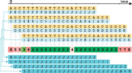
Genotype uncertainty level inference. The figure shows at the top the alignment of four reads. The colored bar in the middle represents the genotype uncertainty at each locus, where dark green represents low uncertainty while red represents high uncertainty. The numbers shown in the middle bar are the indexes k chosen for each locus. The value of k also indicates the number of different quantization levels of its associated quantizer. Finally, the figure shows at the bottom the quantized quality values for the four reads

As an example, at the left-most locus shown in Figure 1, there is not enough evidence for a particular genotype as only two bases cover that position, with one of them having a rather high quality value and the other one of them having a rather low quality value. Thus, the number of different quantized quality values that can appear in that locus will be high, namely k = 8 in this example. On the other hand, the figure also contains several loci with low ‘genotype uncertainty’, highlighted in dark green. In these cases, only two quality values (i.e. k = 2) will be used to represent all quality values at each of these loci. Finally, note that at the fifth genomic locus (l = 4), all bases aligning in that position match perfectly. However, since half of the quality values in that position are low, the ‘genotype uncertainty’ is also increased. This results in an increment of the number of quantization levels that will be used at that locus.

Algorithm 1: CALQ

Data: SAM file and the reference genome with length L

Result: compressed quality values

1 set locus index: $l\leftarrow 0$⁠;

2 whilel < Ldo

3   read all reads covering locus l;

4   extract CIGAR, POS, QUAL and SEQ for each of these reads;

5   compute the genotype uncertainty;

6   compute the index k from the genotype uncertainty;

7   quantize the quality values;

8   $l\leftarrow l+1$⁠;

9 end

10 compress the quantized quality values using an entropy encoder;

11 compress the indexes k using an entropy encoder;

Algorithm 1 shows the set of instructions performed by the proposed algorithm. In words, for every locus l, the encoder gathers the sequences of reads and quality values covering that locus, the read mapping positions, the CIGAR strings and optionally the reference sequence(s), as defined in the SAM file format specification (Li et al., 2009). For each read in the SAM file, its associated CIGAR string is the set of instructions that need to be performed to align the read to the reference, excluding substitutions. Then, CALQ computes the genotype uncertainty at that locus l which is then used to select a specific quantizer with k levels from a previously computed set of quantizers. The chosen quantizer is used to quantize all quality values associated with locus l. Finally, entropy encoders are used to compress the quantized quality values and the indexes k. Supplementary Figure S2 shows the block diagram of the CALQ codec, together with the necessary side information needed for compression and decompression.

Lines 5–7 and lines 10 and 11 from Algorithm 1 are explained in detail in what follows.

2.1 Genotype uncertainty computation

This section describes the computations performed by CALQ to infer the genotype uncertainty (line 5 of Algorithm 1). As mentioned above, the genotype uncertainty is computed from the observable data using a statistical model. In this paper, we use a Bayesian model similar to the one used by the tool UnifiedGenotyper from the Genome Analysis Toolkit (GATK) (McKenna et al., 2010). However, in other implementations, the model could be controlled or selected depending on the targeted application or depending on general preferences of the user.

At any locus l in the sequenced genome, the genotype is represented by a random variable G drawn from the genotype alphabet $\mathcal{G}$ with cardinality $\left|\mathcal{G}\right|$⁠. The genotype G is the set of alleles found at a locus l across all reads covering it. We express the genotype as $G=(A_1,\dots ,A_{\alpha },\dots ,A_h)$⁠, where the allele $A_{\alpha }$ is drawn from the allele alphabet $\mathcal{A}$ with cardinality $\left|\mathcal{A}\right|$⁠, and h is the ploidy of the species. Then we can derive the number of possible genotypes $\left|\mathcal{G}\right|$ by computing all possible allele combinations with repetitions as

$$\left|\mathcal{G}\right|=\left(\begin{array}{c}\left|\mathcal{A}\right|+h-1\\ \left|\mathcal{A}\right|-1\end{array}\right).$$

(1)

For example, in the case of DNA sequencing, we consider the allele alphabet $\mathcal{A}=\left\{\mathrm{A,C,G,T}\right\}$ with $\left|\mathcal{A}\right|=4$ symbols. As an example, for a diploid organism with h = 2, this would result in $\left|\mathcal{G}\right|=10$ possible genotypes. Note that the symbol $\mathrm{N}$ is emitted by a sequencing machine if no decision about a nucleotide at a specific position can be made. However, since real DNA sequences cannot contain symbol $\mathrm{N}$⁠, we omit it here.

Let us consider a set of reads that are aligned to a reference sequence and let us assume that the reads have been sorted by their mapping positions. Given such set of reads, we denote by N the number of reads covering locus l. Let n_i be the symbol from read i covering the locus l and q_i the value of the corresponding quality value.

The goal is to compute the posterior distribution of the genotype G, given the observable nucleotides $\mathbf{n}={\left\{n_i\right\}}_{i=1}^N$ parameterized by the observable quality scores $\mathbf{q}={\left\{q_i\right\}}_{i=1}^N$⁠. The posterior probability is proportional to the likelihood times the prior:

$$P(G|\mathbf{n};\mathbf{q})\propto P(\mathbf{n}|G;\mathbf{q})·P(G).$$

(2)

The likelihood is given by

$$P(\mathbf{n}|G;\mathbf{q})=\prod _{i=1}^{N}P(n_i|G;q_i),$$

(3)

where $P(n_i|G;q_i)$ is the likelihood of having observed n_i given that the genotype was G, parameterized by q_i. Recall that the genotype G is expressed as $G=(A_1,\dots ,A_{\alpha },\dots ,A_h)$⁠, where $A_{\alpha }$ is the α-th allele. Note that the nucleotide n_i was drawn from only one of the alleles. Hence, we give all alleles equal probability of being the one from which the nucleotide n_i was drawn. Thus, the likelihood is given by

$$P\left(n_i|G=(a_1,\dots ,a_h);q_i\right)=\sum _{\alpha =1}^h\frac{P\left(n_i|A_{\alpha }=a_{\alpha };q_i\right)}{h},$$

(4)

where $P(n_i|A_{\alpha }=a_{\alpha };q_i)$ is the likelihood of having observed n_i given the assumption that the true symbol was the allele $a_{\alpha }$⁠, parameterized by q_i. This probability is given by

$$P\left(n_i|A_{\alpha }=a_{\alpha };q_i\right)=\{\begin{array}{cc}1-{10}^{-\frac{q_i}{10}},\hfill & n_i=a_{\alpha }\hfill \\ \frac{{10}^{-\frac{q_i}{10}}}{\left|\mathcal{A}\right|-1},\hfill & n_i\ne a_{\alpha }\hfill \end{array}.$$

(5)

Finally, given the genotype likelihood $P(\mathbf{n}|G;\mathbf{q})$⁠, the genotype uncertainty is calculated by applying the metric $M(P(\mathbf{n}|G;\mathbf{q}))$ over the genotype likelihood. Specifically, we choose M to be one minus the difference between the maximum likelihood ${\mathrm{\mathbb{P}}}_{\text{ML}}$ and the second largest likelihood ${\mathrm{\mathbb{P}}}_2$⁠, i.e.

$$M=1-({\mathrm{\mathbb{P}}}_{\text{ML}}-{\mathrm{\mathbb{P}}}_2).$$

(6)

The difference $({\mathrm{\mathbb{P}}}_{\text{ML}}-{\mathrm{\mathbb{P}}}_2)$ can be interpreted as the genotype certainty (and hence, one minus the genotype certainty yields the genotype uncertainty). Note that any other metric, such as the entropy or the Kullback-Leibler divergence, could also be used. Specifically, we chose the metric M as defined in Equation 6 over the entropy and the Kullback-Leibler divergence because it yields more meaningful results in the case that the genotype likelihood $P(\mathbf{n}|G;\mathbf{q})$ consists of few approximately equally likely genotypes. Finally, by using the likelihood (without the prior) to compute the genotype uncertainty levels, the proposed scheme is able to operate without a reference. However, the posterior could be used instead of the likelihood if a reference is available.

2.2 Quantizer index k computation

We use the already computed genotype uncertainty M to compute the quantizer index k as

$$k\leftarrow f(M(P(\mathbf{n}|G;\mathbf{q}))),$$

(7)

where f is a monotonous increasing function. Specifically, it is a uniform quantization function mapping the possible metric values to an integer set of possible quantization indexes. We configure f to output integer values in the interval $[2,8]$⁠. These values represent the number of quantization levels to be used for the quantization of quality values at the corresponding locus. Hence, in the current implementation, CALQ is preloaded with seven uniform quantizers with two to eight quantization levels. For example, if for a specific locus the computed genotype uncertainty is very low, then CALQ will select the lowest quantization index, namely k = 2. Thus, a uniform quantizer with two quantization levels is selected for that locus.

We chose two quantization levels for the coarsest quantizer, since this binary decision is well suited for loci with a low genotype uncertainty. Given the trend to reduce the quality values resolution, we chose 8 quantization levels for the finest quantizer to mimic Illumina’s 8-binning. In other words, CALQ takes 8-binning as a baseline and at the same time still leaves room for improvement of both the resulting compression rate and the variant calling performance by selecting quantizers with fewer quantization levels when appropriate.

2.3 Quantization

The quantizers transform the input quality values into quantization indexes i. For a quantizer with k uniform quantization levels, the possible output quantization indexes i are in the interval $[0,(k-1)]$⁠. Using the same example as above, after choosing the quantizer index to be k = 2, the quantizer will output the quantization index i = 0 for the low quality values in that locus, and the quantization index i = 1 for those which are high. The threshold that determines what is a low or a high quality value is set by the quantizer.

At the decoder, the quality values have to be reconstructed using the quantization indexes i (in correspondence with the correct quantization tables k). The representative quality values are placed at the mid-points of the corresponding bins.

2.4 Entropy encoder

CALQ processes the input data in fixed-size blocks, where each block contains b sequence alignments. We empirically derived a suitable block size of b = 10 000 sequence alignments using an E.coli DH10B strain dataset, sequenced with Illumina (i.e. short-read paired-end) technology at a coverage of 422×. For more details on the selection of the block size, we refer the reader to the Supplementary Material.

The quantization indexes i outputted by the quantizers are encoded with seven order-0 arithmetic encoders (Witten et al., 1987), selected by the corresponding quantizer index k. In other words, the seven arithmetic encoders model the seven conditional probability distributions $P(i|k)$⁠. The quantizer indexes k are encoded with another order-0 arithmetic encoder, which models the probability distribution P(k). All arithmetic encoders work non-adaptively, i.e. they accumulate the individual symbol probabilities of a block of data before performing the actual compression. The outputs (including the accumulated probabilities) of all entropy coders are then multiplexed and written to the output file. Note that to reconstruct the quality values at the decoder, the mapping positions, the CIGAR strings and the reference sequence(s) are required by the decoder. These can be provided by an existing SAM/BAM compressor [for example CRAM (Bonfield, 2014; Hsi-Yang Fritz et al., 2011) or TSC (Voges et al., 2016)].

3 Results and discussion

We start this section by showing how the genotype uncertainty correlates with the sequencing depth. To that end, we computed the genotype likelihood as specified in the Materials and methods (Section 2.1) on an E.coli DH10B strain dataset with an average sequencing depth (i.e. coverage) of 422×. Note that in this case the organism is haploid, thus, h = 1.

Figure 2 shows the sequencing depth (blue, top curve) and the genotype certainty (yellow, bottom curve) for the first 1000 loci. For ease of visualization, we computed the genotype certainty as the negative decimal logarithm of the entropy of the genotype likelihood, i.e. $-{\text{log}}_{10}\hspace{0.17em}H(P(\mathbf{n}|G;\mathbf{q}))$⁠. As shown in the figure, the genotype certainty curve accurately follows the sequencing depth one. This is to be expected, as more sequencing depth at a given locus yields more information to estimate the genotype. As observed in the figure, the genotype uncertainty is extremely low at most loci (high values in the figure). In these cases, the quality values could be highly compressed as they will likely play a minor role in determining the genotype at these loci.

Fig. 2.

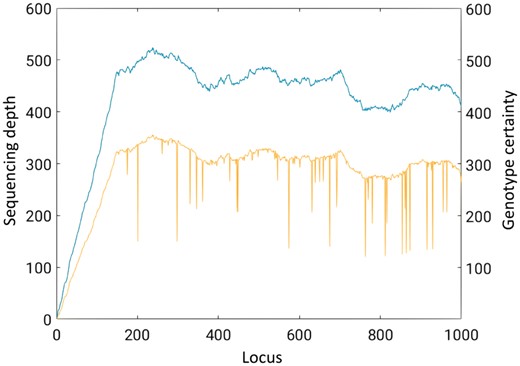
Sequencing depth (blue, top curve) and genotype certainty (yellow, bottom curve) for the first 1000 loci of the E.coli DH10B strain. For ease of visualization we plot the genotype certainty instead of the genotype uncertainty (Color version of this figure is available at Bioinformatics online.)

However, for a few loci deep narrow valleys are observed. These represent those loci where the genotype uncertainty is high (low values in the figure). Hence, the quality values will play an important role in the computation of the genotype at these loci. In these cases, by applying finer quantization, the quality values will remain very close to the original ones.

3.1 Impact on variant calling

Since CALQ is a compressor where the reconstructed (i.e. decompressed) quality values can be different from the original ones, it is of uttermost importance to assess the effect that these changes in the quality values have on downstream applications. In the scope of this paper, we choose variant calling as it is crucial for clinical decision making and thus widely used.

We selected three different variant calling pipelines. The first pipeline is composed by the GATK Best Practices pipeline (DePristo et al., 2011). Moreover, this pipeline is used in the MPEG initiative for the standardization of genomic information representation (Alberti et al., 2016). Its last step consists of filtering the called variants to remove possible false positives. Although the GATK Best Practices call for the use of the Vector Quality Score Recalibration (VQSR) method, to the knowledge of the authors this is still not widely adopted. Hence, we also consider the more traditional hard filtration of variants as the second pipeline. The third pipeline consists of the variant caller Platypus as presented in (Rimmer et al., 2014).

The outputs of all pipelines are analyzed using the hap.py benchmarking tool as proposed by Illumina and adopted by the Global Alliance for Genomics and Health (GA4GH, https://github.com/ga4gh/benchmarking-tools).

We refer to the Supplementary Material accompanying this paper for the specific commands and parameters used in these pipelines.

The datasets used for this analysis pertain to the same individual, namely NA12878. The reason behind this choice is that the National Institute of Standards and Technology (NIST) has released a consensus set of variants for this individual (Zook et al., 2014). With the publication of this consensus set we have the means for analyzing, in a more concise manner, the effect that lossy compression of quality values has on variant calling. Note that similar analyses were conducted in other works (Alberti et al., 2016; Ochoa et al., 2016).

Figure 3 shows the scheme of the used pipelines for the analysis. The box shown in the middle of the figure is where each of the analyzed lossy compressors will transform the quality values. To generate the metrics that will be used as baseline (i.e. the lossless results) the same pipeline is used but with the green box removed.

Fig. 3.

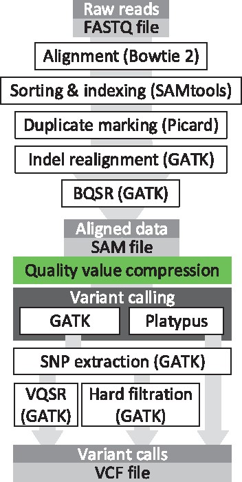
The variant calling pipelines used for the performance assessment of the proposed lossy compressor CALQ

Although in Ochoa et al. (2016) and Alberti et al. (2016) an argument was made to perform the lossy compression at the beginning of the pipeline, we believe that placing it just before the variant calling is a more realistic position since it is the point where all processing of the SAM file has been done. We believe that if one would need to store a SAM file, it would be the one at this point, after all processing, and not the ones before, which have been subject to less processing.

After each run of the pipeline, a set of variants is obtained which are stored in the well-known VCF file format. Note that when using the GATK + VQSR pipeline, in the last step, a filter level must be specified such that all variants below that filter value are discarded. Specifically, and similar to Ochoa et al. (2016) and Alberti et al. (2016), we have chosen to use four different levels of filtering, namely (and ordered from more to less restricting) 90, 99, 99.9 and 100. For more information about the meaning of this filter values and the specific filters of the other pipelines we refer the reader to the Supplementary Material.

Afterwards, each set of variants (stored in the output VCF file) is compared against the consensus set of variants released by the NIST. This comparison is performed using the benchmarking tool hap.py. Note that a BED file is also used to restrict the comparison to the high-confidence regions of the consensus set.

The benchmarking tools output the following values.

• True Positives (T.P.): All those variants that are both in the consensus set and in the set of called variants.

• False Positives (F.P.): All those variants that are in the called set of variants but not in the consensus set.

• False Negatives (F.N.): All those variants that are in the consensus set but not in the set of called variants.

• Non-Assessed Calls: All those variants that fall outside of the consensus regions defined by the BED file. This distinction was not considered in previous papers by Malysa et al. (2015), Ochoa et al. (2016), Alberti et al. (2016) and Yu et al. (2015), where all these variants were accounted as positives, and therefore inflating the false positives metric. This could be the reason behind the bad performance of the variant callers seen in the mentioned works.

These values are used to compute the following two metrics:

• Recall/Sensitivity: This is the proportion of called variants that are included in the consensus set; that is, $R=\mathrm{T}.\mathrm{P}./(\mathrm{T}.\mathrm{P}.+\mathrm{F}.\mathrm{N}.)$⁠,

• Precision: This is the proportion of consensus variants that are called by the variant calling pipeline; that is, $P=\mathrm{T}.\mathrm{P}./(\mathrm{T}.\mathrm{P}.+\mathrm{F}.\mathrm{P}.)$⁠.

We use these metrics to assess the performance of CALQ, as well as the performances of previously proposed algorithms.

We start by assessing the performance of the proposed algorithm using the GATK Best Practices pipeline as proposed by the Broad Institute, which includes VQSR as the variant filtering step.

For the first set of simulations we used the paired-end run ERR174324 of the NA12878 individual. This run was sequenced by Illumina on an Illumina HiSeq 2000 system as part of their Platinum Genomes project. The coverage of this dataset is 14×. Following the approach of Ochoa et al. (2016) we consider chromosomes 11 and 20. In addition to using chromosomes 11 and 20, to broaden our test set, we also considered chromosome 3.

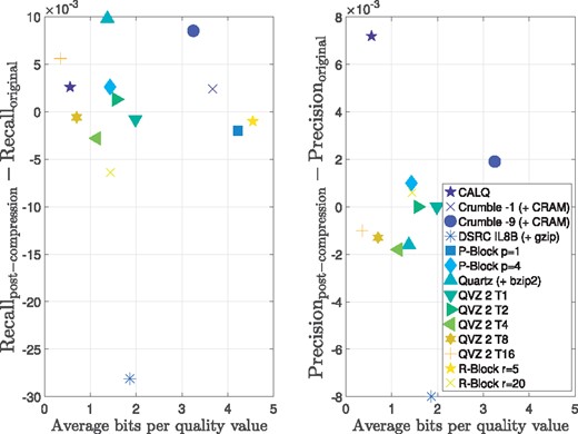
Figure 4 shows the bits per quality value versus the average Recall and Precision over the considered variant calling pipeline achieved by the proposed algorithm CALQ, and by Crumble (for two different modes) (https://github.com/jkbonfield/crumble), Illumina binning (performed with DSRC) (Deorowicz and Grabowski, 2011), P-Block (for two different modes) (Cánovas et al., 2014), Quartz (Yu et al., 2015), QVZ 2 (for five different compression modes) (Hernaez et al., 2016) and R-Block (for two different modes) (Cánovas et al., 2014). We refer the reader to the Supplementary Material for brief descriptions of these tools. The values shown in the figure are the result of averaging over the four VQSR filtering values mentioned above as well as over all three chromosomes. For the individual values for each filter and chromosome we refer to the Supplementary Material.

Fig. 4.

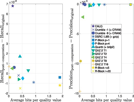
Recall and Precision results for the Illumina HiSeq 2000 dataset ERR174324 with a coverage of 14×. The Recall and Precision metrics were averaged over the four VQSR filtering values as well as over all chromosomes 3, 11 and 20

From the figure we can observe that CALQ achieves the best performance in terms of both Recall and Precision. Moreover, CALQ achieves a considerably higher average Recall than that of the lossless case. This means that the variant caller identifies more true positives with CALQ quality values than with the original ones. Note that this is also true for some of the other lossy compressors, although in a minor scale. This seems to indicate that by applying a lossy compressor, more true positives are discovered. These results may seem surprising, however, similar findings for different lossy compressors were found by Alberti et al. (2016), Ochoa et al. (2016) and Yu et al. (2015).

Regarding the Precision, CALQ also achieves the best results, yielding a performance marginally above the lossless case. This improvement with respect to the lossless case is also observed for 7 out of the other 13 compressors. However, all incur in more bits per quality value. In this regard, CALQ achieves a compressed size of less than 0.2 bits per quality value which is an order of magnitude less than the state-of-the-art lossless compressors.

Next, we show the results for the SRR1238539 run on the NA12878 individual for which an Ion Torrent sequencing machine was used. The coverage of this dataset is 10×. As before, chromosomes 3, 11 and 20 were considered. Again, the results shown are the results of averaging over the same four filter values and both chromosomes.

Figure 5 shows the results for the Ion Torrent dataset. As before, we run the analysis using 14 different compressors (including the different modes for some lossy compressors) and computed the Recall and Precision.

Fig. 5.

Recall and Precision results for the Ion Torrent dataset SRR1238539 with a coverage of 10×. The Recall and Precision metrics were averaged over the four VQSR filtering values as well as over all chromosomes 3, 11 and 20

As seen in the figure, for the case of Recall, Quartz is the best-performing algorithm. However, it performs among the worst in terms of Precision. This is probably due to the fact that, on average, more calls are made on Quartz compressed data than on the original data. However, these extra calls are also filled with false positives, as shown by the performance drop on Precision incurred by the Quartz compressed data.

Regarding the proposed algorithm CALQ, the Recall performance is comparable to the best modes of the different compressors. However, in terms of Precision, CALQ yields a significant improvement over the rest of the algorithms, including the original dataset. Finally, note that the Illumina binning as implemented by DSRC performs very poorly in both Recall and Precision.

Next, Supplementary Figure S9 shows the results for the sample dataset generated by the Garvan Institute from the Coriell Cell Repository NA12878 reference cell line. These data were sequenced on a single lane of an Illumina HiSeq X machine. The coverage of this dataset is 49×.

In this case, all compression modes except P-Block with p = 4 achieve better Recall than the original. In terms of Precision, the proposed algorithm lies in the Precision-size trade-off curve. For more data on the results for the individual filter values and chromosomes, we refer to the Supplementary Material.

To conclude this assessment, Figures 6 and 7 show the Precision and Recall difference between using the original data and the lossy-compressed data for the three pipelines considered in this paper. We depict $54=6\times 3\times 3$ points per lossy compressor, which are the results of running 6 different pipelines (GATK + hard filtration, Platypus and 4 different filter values for GATK + VQSR), using the above mentioned 3 datasets and 3 chromosomes (3, 11 and 20) for each dataset. The x-axes show the average compression ratio of each of the analyzed methods with respect to the losslessly compressed quality values sizes in the BAM files. The individual points were jittered along the x-axes for clarity. For example, a compression ratio of 10% means that the lossy compressed quality values consume 10% of the quality value sizes in the BAM files. The figures also show the aggregated results in form of a box plot showing the mean (red line), the 95% standard error of the mean (red box) and the standard deviation (blue whiskers). Note, that we excluded the results for P-Block p = 1 and R-Block r = 5 from both figures, since their compression ratios are at 76 and 80% with respect to BAM, hampering a clear presentation of the results. We therefore refer the reader to the Supplementary Material for these results.

Fig. 6.

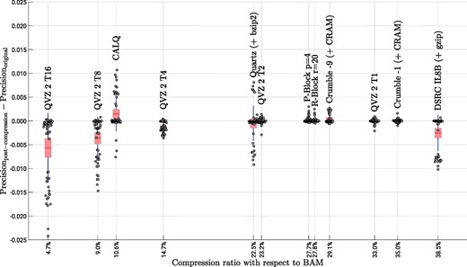
Precision results for all considered pipelines, datasets and chromosomes. A total of 54 individual points are shown for each of the lossy compression methods. The data is aggregated in form of a box plot showing the mean (red line), the 95% standard error of the mean (red box) and the standard deviation (blue whiskers) (Color version of this figure is available at Bioinformatics online.)

Fig. 7.

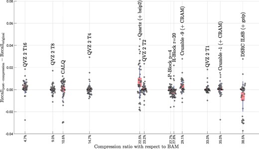
Recall results for all considered pipelines, datasets and chromosomes. A total of 54 individual points are shown for each of the lossy compression methods. The data is aggregated in form of a box plot showing the the mean (red line), the 95% standard error of the mean (red box) and the standard deviation (blue whiskers) (Color version of this figure is available at Bioinformatics online.)

We first focus our attention on the Precision results shown in Figure 6. For QVZ 2, a high variance can be observed for the high-compression modes T8 and T16. In these cases, there are few instances in which the lossy compressed data achieve better or similar performance to that of the original data, whereas in most instances there is a clear deterioration in performance. A similar behavior can be observed for Quartz, although with less variance and slightly better results than those of QVZ 2 T8 and T16. However, with 22.5% on average, the compression ratio achieved by Quartz is significantly larger.

For the low-compression modes of QVZ 2 (i.e. T1, T2 and T4), for P-block, R-Block and for Crumble (both modes) the results are quite consistent (low variance) and very similar to those of the original data. In these cases, the compression ratios vary from 23.2% (QVZ 2 T2) to 35.0% (Crumble -1).

The proposed algorithm CALQ achieves a variance similar to that of Quartz, but in almost all instances the performance of CALQ-compressed data outperforms that of the original data, being the only method to boost performance. In terms of compression ratio, CALQ achieves an average of about one order of magnitude (10.6%) reduction in size with respect to BAM compressed data. Furthermore, its performance is considerably better than that of the two other methods (QVZ 2 T8 and T16) that achieve better compression ratios.

The Illumina binning is the worst performing method of all. It achieves the worst compression rate while yielding a high variance and overall poor results.

Interestingly, the results for Recall, which are shown in Figure 7, are quite different in terms of results variance and performance. Here, all compressors yield similar variances with Quartz being the one with the highest variance, and the high-compression modes of QVZ 2 and P-Block and R-Block being the ones with the lowest variance. Regarding the variant calling performance, almost all methods in nearly all cases outperform the original data, with Quartz being the one achieving an overall best Recall. The proposed method performs very similarly to the other methods while achieving higher compression gains. Again, the Illumina binning is the worst performing method of all, achieving an overall poor performance.

Finally, due to the heuristic nature of the variant calling pipelines, it is hard to separate the effect that the different confounding factors have on the final results. This hampers considerably the ability for a deeper analysis on which particular conditions yield an improvement on variant calling. However, as hypothesized by Ochoa et al. (2016), we believe that the proposed lossy compressor produces partially denoised quality values that, under most conditions, improve the accuracy of the variant calling pipeline.

3.2 Compression performance on non-human datasets

Finally, in addition to the three human datasets, we tested the compression performance of CALQ on an E.coli DH10B strain dataset, sequenced with Illumina (i.e. short-read paired-end) technology. This dataset was sequenced at a coverage of 422×. Furthermore, we tested CALQ on a fifth dataset, which is a D. melanogaster genome sequenced with Pacific Biosciences (i.e. long-read) technology at a coverage of 100×. The complete compression results in bits per quality value for all five datasets are shown in Table 1.

Table 1.

CALQ compression ratios in bits per quality value (bits/QV) for the five considered datasets

Dataset	Species	Coverage	Compression ratio
ERR174324	H.sapiens	14×	0.15 bits/QV
SRR1238539	H.sapiens	10×	0.56 bits/QV
Garvan replicate	H.sapiens	49×	0.46 bits/QV
DH10B	E.coli	422×	0.30 bits/QV
dm3	D.melanogaster	100×	0.16 bits/QV

We can observe from the table that the coverage is correlated with the compression ratio. This is to be expected since generally a higher sequencing depth at a given locus yields a higher genotype certainty for that locus. CALQ exploits this effect by quantizing the quality values at these loci using quantizers with very few levels. Furthermore, the outputs of these quantizers are highly compressible yielding superior compression ratios. For example, the best compression ratio from Table 1 is 0.15 bits per quality value for the dataset ERR174324. This result suggests that this particular dataset contains few errors since high genotyping certainty values are computed by CALQ for almost all loci.

3.3 Computational performance

Regarding the computational performance of each of the methods, CALQ uses the least memory of all of them while maintaining a reasonable processing time, operating on average at 0.5 MB/s during encoding and 3.3 MB/s during decoding, respectively. The CALQ encoder yields an average peak memory usage of approximately 90 MB and the CALQ decoder even uses only about 20 MB of RAM. QVZ 2 and Crumble (in all their modes) exhibit average peak memory usages of approximately 3.7 GB and 54 MB, respectively. P- and R-Block use around 700 MB of RAM. However, due to its memory-expensive algorithm, Quartz (run in its low-memory mode) yields an average peak memory usage of 26 GB which hampers its application on most personal computers and embedded devices. We refer to Section 3 of the Supplementary Material for a deeper analysis of the performances of the used compressors, including CALQ.

4 Conclusion

In this paper, we propose the first lossy compressor for quality values that exploits the alignment information contained in the SAM/BAM files. Specifically, CALQ computes a genotype certainty level per genomic locus to determine the acceptable coarseness of quality value quantization for all the quality values associated to that locus.

We analyze the performance of several lossy compressors for quality values in terms of trade-off between the achieved compressed size (in bits per quality value) and the Precision and Recall achieved after running three different variant calling pipelines over sequencing data of the well-known individual NA12878. By compressing and reconstructing quality values with CALQ, we observe a better average variant calling performance than with the original data. At the same time, with respect to the state-of-the-art lossless compressors, CALQ achieves a size reduction of about one order of magnitude, yielding only 0.37 bits per quality value on average. This is approximately a 10-fold improvement of the compression factor with respect to BAM. The better variant calling performance is not a surprising fact as it has been previously validated for other lossy compressors in the past. However, previously proposed lossy compressors fail to achieve an order of magnitude improvement in compression.

Furthermore, we show that CALQ performs as good as or better than the state-of-the-art lossy compressors in terms of Recall and Precision for most of the analyzed datasets.

Finally, we further validate previous work that showed that the binning performed by Illumina is far from being the best approach for reducing the burden that the quality values have on the size of SAM/BAM files.

Funding

This work has been partially supported by the Leibniz Universität Hannover eNIFE grant, the Stanford Data Science Initiative (SDSI), the National Science Foundations grant NSF 1184146-3-PCEIC and the National Institute of Health grant with number NIH 1 U01 CA198943-01.

Conflict of Interest: none declared.