K  ₂ and $K2*$⁠: efficient alignment-free sequence similarity measurement based on Kendall statistics

Abstract

Motivation

Alignment-free sequence comparison methods can compute the pairwise similarity between a huge number of sequences much faster than sequence-alignment based methods.

Results

We propose a new non-parametric alignment-free sequence comparison method, called K₂, based on the Kendall statistics. Comparing to the other state-of-the-art alignment-free comparison methods, K₂ demonstrates competitive performance in generating the phylogenetic tree, in evaluating functionally related regulatory sequences, and in computing the edit distance (similarity/dissimilarity) between sequences. Furthermore, the K₂ approach is much faster than the other methods. An improved method, $K_2^{*}$⁠, is also proposed, which is able to determine the appropriate algorithmic parameter (length) automatically, without first considering different values. Comparative analysis with the state-of-the-art alignment-free sequence similarity methods demonstrates the superiority of the proposed approaches, especially with increasing sequence length, or increasing dataset sizes.

Availability and implementation

The K₂ and $K_2^{*}$ approaches are implemented in the R language as a package and is freely available for open access (http://community.wvu.edu/daadjeroh/projects/K2/K2_1.0.tar.gz).

Supplementary information

Supplementary data are available at Bioinformatics online.

1 Introduction

Evaluating the similarity between two sequences is a classical problem that has long been studied in computer science, primarily from the view point of string pattern matching (Adjeroh et al., 2008; Gusfield, 1997). Such similarity measurement has applications in various areas in computational biology, e.g. sequence alignment (Smith and Waterman, 1981), in comparative genomics (Aach et al., 2001), genomic evolution and phylogenetic tree construction and analysis (Cao et al., 1998; Reyes et al., 2000), analysis of regulatory functions (Kantorovitz et al., 2007), rapid search in huge biological sequences (Wandelt and Leser, 2013). Other recent applications include compression and efficient storage of the rapidly expanding genomic datasets (Beal et al., 2016a, b; Deorowicz and Grabowski, 2013; Giancarlo et al., 2012), and resequencing a set of strings given a target string (Kuo et al., 2015), an important step in efficient genome assembly.

Alignment-free sequence comparison methods can compute the similarity between a large number of sequences much faster than alignment-based methods (Vinga and Almeida, 2003; Vinga, 2014). Word analysis of k-length substrings (also called k-mers, k-grams, or k-tuple) from sequences is one approach to improved sequence comparision (Bonham-Carter et al., 2014). Words can be extracted in different ways, and with varying lengths. The most common is to use sliding windows from length 2 to n – 1, where n is the length of sequence (Bauer et al., 2008; Dai et al., 2011; Liu et al., 2006; Qi et al., 2004). Some methods divide a sequence into several even parts (Zhao et al., 2011), while some others have used fixed length substrings, e.g. k = 2 (2-mer) (Shi and Huang, 2012). After extracting the words, different statistical methods can be applied to analyze two sequences for similarity (Li and Wang, 2005; Wang and Zheng, 2008). DMk (Wei et al., 2012) and Category-Position-Frequency (CPF) (Bao et al., 2014) incorporate positions and frequencies of k-mers into feature vectors. DV (Zhao et al., 2011) utilizes distribution vectors from k-mers. Shi (Shi and Huang, 2012) maps a DNA primary sequence into three symbolic sequences and groups these sequences into a twelve-component vector. Wavelet Feature Vector (WFV) converts a sequence into a L-length feature vector by wavelet transform (Bao and Yuan, 2015).

Our approach is more closely related to the D₂ statistic, another popular approach for measuring the similarity (or dissimilarity) between two sequences (Bonham-Carter et al., 2014; Song et al., 2014). It was first proposed by Blaisdell (1986). Since then, many variants and improvements have been proposed, such as $D_2^z$ (Kantorovitz et al., 2007), $D_2^{*}$ (Reinert et al., 2009) and $D_2^{sh}$ (Wan et al., 2010). $D_2^z$ (Kantorovitz et al., 2007) normalizes the D₂ statistic using its mean and standard deviation to improve its detection power (Song et al., 2014). $D_2^{*}$ and $D_2^{sh}$ are two other normalization improvement methods which were proposed in Reinert et al. (2009) and Wan et al. (2010). $D_2^{sh}$ [also denoted $D_2^S$ in the literature (Reinert et al., 2009; Song et al., 2014)] uses an approach based on Shepp (1964). According to a recent review (Song et al., 2014), $D_2^{sh}$ and its variant are generally the best D₂ statistical methods for alignment-free comparison of genomic sequences, especially with increasing sequence length. More detailed discussion of the D₂-statistic family of algorithms can be founded in Section 6 of the Supplementary Material.

In general, the D₂-statistic family of algorithms have a general problem of requiring a quadratic or cubic time complexity, with respect to n or m, the length of the sequences, and k, the size of the substrings being considered. Also, the D₂ family of statistics generally makes some assumptions on the distribution of the sequences, for instance, most assumed either a uniform distribution, or a normal distribution, for the symbols in the sequences. This parametric nature of the statistics obviously limits their practical applicability, since practical data, especially for biological sequences (e.g. complete genomes for individuals of the same species, or for related organisms) rarely follow these theoretical distributions. A non-parametric approach to the measurement of sequence similarity is required, one that does not make any assumption on the distribution of the sequences under consideration, and one that is efficient enough to handle the rapidly increasing complexity and data sizes of available biological sequence data.

In this work, we propose a nonparametric approach, K₂, which uses the Kendall correlation statistic to estimate the similarity between sequences. The Kendall correlation is a non-parametric method to calculate the correlation between two sets of random variables. We adopt this to measure the similarity among sequences. When compared to the other state-of-the-art alignment-free sequence similarity methods, (e.g. D₂, $D_2^{*},\hspace{0.17em}{D}_2^{sh},\hspace{0.17em}{D}_2^z$⁠, DMk, DV, CPF, Shi and WFV), K₂ demonstrates an improved power in detecting relatedness between sequences, as measured by its ability to generate the correct phylogenetic tree, and to identify functionally related regulatory sequences. The K₂ also showed significant correlation with the edit distance, the standard, though time consuming, measure of (similarity/dissimilarity) between sequences. Further, the K₂ approach is faster than most of the other methods when k is large, (typically, with $k\ge 7$⁠). This places the proposed K₂ statistic among the best non-alignment based similarity measures, especially with increasing sequence lengths (n, m), or increasing size of the k-mer. Based on K₂, we further propose an improved method, named $K_2^{*}$⁠, which is able to determine a suitable value for k, the k-gram parameter automatically with competitive performance. We have implemented K₂ and $K_2^{*}$ in the R statistical and graphics environment, and the codes are freely available for open access.

2 Materials and methods

2.1 Kendall statistic

The Kendall statistic is a nonparametric method which makes no assumption about the probability distribution of the variables being assessed. The Kendall statistic estimates the correlation between two sets of random variables X and Y, represented using the pairs $(X_1,Y_1)(X_2,Y_2)\dots (X_n,Y_n)$⁠. The Kendall correlation, τ, is then defined as follows (Kendall, 1938).

$$\tau (X,Y)=P\left\{\right(X_j-X_i\left)\right(Y_j-Y_i)>0\}-P\left\{\right(X_j-X_i\left)\right(Y_j-Y_i)<0\}$$

(1)

In this study, we compute the Kendall correlation by using the following formula to approximate τ (Kendall, 1938; Marden et al., 1992):

$$\widehat{\tau }=\frac{n_c-n_d}{\frac{n\times (n-1)}{2}}$$

(2)

where n is the number of distinct k-grams for the concatenated sequence S=$T\$P\$$⁠, $n_c$ is the number of concordant $k$-gram pairs $(X_j-X_i)(Y_j-Y_i)>0$⁠, with $0<i<j\le n$⁠; and $n_d$ is the number of discordant $k$-gram pairs $(X_j-X_i)(Y_j-Y_i)<0$⁠, with $0<i<j\le n$⁠.

2.2 Optimized computation of Kendall statistics

The time cost to compute $\widehat{\tau }$⁠, the approximation to the Kendall correlation statistic is $O\left(n^2\right)$⁠, including time to compare each pair between (⁠$X_i,X_j$⁠) and (⁠$Y_i,Y_j$⁠), $i\ne j$⁠, where $n$ is the number of pairs in $X$ and $Y$⁠. Christensen (2005) showed an algorithm to calculate $\widehat{\tau }$ in $O(n\hspace{0.17em}\text{log}\hspace{0.17em}n)$ time complexity. It was implemented in Pascal. Lin et al. (2017) recently introduced an algorithm for the related problem of weighted Kendall correlation. In this work, we propose data structures and a new algorithm to compute $\widehat{\tau }$⁠. Our algorithm also runs in $O(n\hspace{0.17em}\text{log}\hspace{0.17em}n)$ time, but uses a different approach to compute the Kendall statistics. We then apply the algorithm to analyze similarity between a given pair of sequences. More detailed discussion on the improved algorithm for the Kendall Statistics can be found in Section 3.1 of the Supplementary Material.

2.3 The $K_2$ approach

Here, we propose the $K_2$ statistic as a new method for rapid and efficient measurement of biological sequence similarity, without requiring an initial sequence alignment step. The $K_2$ statistic makes use of the above optimized method for computing the Kendall’s $\tau$ correlation between two sequences. Here, the correlation is computed based on the $k$-mer count statistics $(X_{\mathbf{w}}$ and $Y_{\mathbf{w}})$ between the two sequences. The counts are obtained in $O\left(\right|S\left|\right)$ time using the suffix array data structure (Adjeroh et al., 2008; Gusfield, 1997; Manber and Myers, 1993), where $\left|S\right|$ is the length of input sequence $S=T\$P\$$⁠. We describe the steps of the algorithm in the following.

1. Given two sequences T and P, combine them into one sequence, $S=T\$P\$$⁠, after appending an ‘$\$$’ at the end of each sequence. The concatenated sequence S is of length $\left|S\right|$⁠.

2. Build the suffix array (SA) from the combined sequence $S=T\$P\$$⁠. And for a given parameter $k$⁠, read all $k$-grams from SA.

3. Compute the frequency for each $k$-gram using the SA. Here, we use $X_{\mathbf{w}}$⁠, and $Y_{\mathbf{w}}$ to denote the frequency of the $k$-gram $\mathbf{w}$ in sequences $T$ and $P$⁠, respectively. Notice that, both $X_{\mathbf{w}}$ and $Y_{\mathbf{w}}$ will be found at essentially the same time, using the SA of the concatenated sequence, $S$⁠.

4. Order all the (⁠$X_{\mathbf{w}},\hspace{0.17em}{Y}_{\mathbf{w}}$⁠) frequencies of $k$-gram pairs by grouping them according to $Y_{\mathbf{w}}$⁠, and then $X_{\mathbf{w}}$⁠. We get pairs {$(X_1,Y_1),(X_2,Y_2),\dots (X_i,Y_i),$$\dots (X_n,Y_n)$}, where $n$ is the number of distinct $k$-grams from the concatenated sequence $S=T\$P\$$⁠, and (X_i, Y_i) is the frequency pair of ith ranked k-gram from sequences T and P. Thus, (1) $Y_i\le Y_{i+1}$ and i < n and (2) $X_i\le X_{i+1}$ when $Y_i=Y_{i+1}$ and i < n.

5. Compute n_c, the number of concordant pairs, and n_d the number of discordant pairs, for the ranked frequency pairs from sequences T and P. The number of concordant pairs n_c is the sum of the number pairs in one of these two conditions: (1) x_i < x_j and y_i < y_j; (2) x_i > x_j and y_i > y_j, where $0\le i<j<n$⁠. Similarly, the number of disconcordant pairs n_d, is the sum of the number of pairs in one of the following two conditions: (1) x_i < x_j and y_i > y_j; (2) x_i > x_j and y_i < y_j, where $0\le i<j<n$⁠.

6. Calculate the Kendall correlation using the formula:

   $$\widehat{\tau }=\frac{n_c-n_d}{\frac{n\times (n-1)}{2}}.$$

7. Return $\widehat{\tau }$ which is the K₂ similarity between sequences T and P.

The last three steps are based on the optimized Kendall algorithm introduced previously (Section 2.2).

2.4 $K_2^{*}$⁠: improved K₂ with automated k value

Similar to the alignment-free methods from the D₂ family, the proposed K₂ approach depends critically on the length parameter, k. Here, we propose a method to determine the k parameter automatically, without needing to test with all possible values.

Given the alphabet $|\Sigma |$ and the length parameter k, there are at most $|\Sigma {|}^k$ possible k-grams, independent of the sequence lengths n and m. These are the unique k-grams, given the alphabet. Given the concatenated sequence $S=T\$P\$$ with length of $\left|S\right|$⁠, the $k$-grams are simply $k$-length substrings of $S$⁠. Thus, we can have at most $\left|S\right|-k+1$ number of $k$-grams from $S$⁠. These may not be unique, since they may include repeated $k$-grams, depending on the nature of the sequences $T$ and $P$⁠. At the same time, we need the $k$-grams to capture most of the variations in the input sequences (now contained in $S$⁠), while avoiding $k$-grams that are repeated inside other $k$-grams. That is, we want the maximal length $k$-grams that capture the variations in $S$⁠, without missing out on the smaller $k$-grams, especially those that did not occur inside the longer $k$-grams. These shorter $k$-grams are likely to be more numerous, and can also provide important information about the sequences. To satisfy the above competing conditions, the choice of $k$ should meet the following criterion:

$$|\Sigma {|}^k\ge |S|-k+1>|\Sigma {|}^{k-1}$$

(3)

where $\left|S\right|=m+n+2$ is the length of the concatenated sequences $S$⁠. Following the above, the value of $k$ can be approximated as:

$$k=\lceil \hspace{0.17em}{\text{log}}_{|\Sigma |}\left(\right|S\left|\right)\rceil$$

(4)

We can observe the connection between the above relation for $k$ and the longest common prefix (LCP) between suffixes in $S$⁠. For an arbitrary sequence $Q$ with symbols from the alphabet $\Sigma$⁠, it is known that, on average, the length of the longest common prefix between suffixes in $Q$ is in $O(\hspace{0.17em}{\text{log}}_{|\Sigma |}(\left|Q\right|\left)\right)$⁠. See Karlin et al. (1983) and Léonard et al. (2012). Thus, for an arbitrary sequence, our suggested value for $k$ is essentially in the same order as this expected maximal LCP value. This makes sense, in that, the maximal length $k$-gram should be close to the expected maximal LCP length, since if we have $k$ values much larger than the average maximal LCP length, we may not be able to observe some repeated $k$-grams. On the other hand, if we use $k$ values much smaller than the average maximal LCP length, we will be double-counting some smaller repeated substrings. Thus, operating with $k$ values far from the expected maximal LCP length could lead to either underestimating or overestimating the frequency for the $k$-grams that capture the major variations in the sequence.

2.5 Comparative complexity analysis

The proposed $K_2$ algorithm runs in $O\left(\right|S|\hspace{0.17em}\text{log}\hspace{0.17em}|S\left|\right)$ time, which is a significant improvement in complexity, when compared with the $O\left(k\right|S\left|\right|\Sigma {|}^k)$ required for computing $D_2$ and other related statistics, or even with the observed improvement that reduces the time to $O\left(k\right|S{|}^2)$⁠. $K_2^{*}$ requires just a one-time run of $K_2$⁠, using the automatically computed $k$-parameter. This will be practically faster than using $K_2$⁠, however, the time complexity of $K_2^{*}$ still remains the same $O\left(\right|S|\hspace{0.17em}\text{log}\hspace{0.17em}|S\left|\right)$ as in $K_2$⁠. More detailed discussion can be found in Section 3.2 of the Supplementary Material.

2.6 Experimental design

To test the proposed methods, we performed some experiments using three different datasets. We also compared our experimental results with those from state-of-the-art alignment-free sequence similarity measurement algorithms.

2.6.1 Datasets and environment

We use three sets of biological sequence data for the experiments in this study. The first dataset used is the complete mtDNA sequences from Cao et al. (1998) and Reyes et al. (2000) containing data on 12 proteins encoded in the H strand of mtDNA in 20 eutherian species. The sequence lengths ranged from 16 300 to 17 080 symbols. This dataset is often used to evaluate the similarity of different species, especially using phylogenetic trees. We call this the ‘mtDNA20’ dataset.

The second dataset is 23 whole mitochondrial DNA genomes from different Eukaryotic fish species of the suborder Labroidei, taken from Fischer et al. (2013). We could not locate the sequences for two of the species, namely, P.trewavasae and T.moorii. Thus, though the original work in Fischer et al. (2013) used 25 species, our dataset contained only 23 of the 25 species. The sequence lengths ranged from 16 440 to 17 040 symbols. We call this dataset the ‘Fish23’ dataset.

The third dataset used is the set containing cis-regulatory modules (CRMs) used by Kantorovitz et al. (2007) in their work on identification of functional relationships between cis-regulatory sequences. There are seven sets including 185 CRM sequences, taken from Drosophila melanogaster and Homo sapiens. We call this the ‘CRM185’ dataset. This dataset is available for download at http://veda.cs.uiuc.edu/d2z/publicdata.tar.gz.

The experiments were performed in a PC environment, running Intel i5, 4 cores, with 16 GB RAM and 1 TB HD. $K_2$ and $K_2^{*}$ were written using the R Language. For comparison purposes, we also tested several other state-of-the-art alignment-free methods using the same datasets. The algorithm for $D_2$ was from Song et al. (2014), $D_2^{sh}$ was from Wan et al. (2010), and $D_2^{*}$ was from Reinert et al. (2009). They all were implemented using the C language. The method $D_2^z$ was developed in Perl in the original work of Kantorovitz et al. (2007). We implemented the methods for $DMk$ (Wei et al., 2012), $CPF$ (Bao et al., 2014), $DV$ (Zhao et al., 2011) and $Shi$ (Shi and Huang, 2012) in R, according to descriptions provided in the respective papers. The codes for $WFV$⁠, developed in Python in their original work (Bao and Yuan, 2015), were kindly provided by the authors. In our experiments, the parameter $k$ corresponds to the length $L=4^k$ in their work.

2.6.2 Experiment 1

The first experiment aimed at analyzing the general performance of each alignment-free method studied. The experiment compared eleven alignment-free methods, namely, $D_2,D_2^{*},D_2^z,\hspace{0.17em}{D}_2^{sh}$⁠, $DMk,\hspace{0.17em}DV,\hspace{0.17em}CPF,\hspace{0.17em}Shi$ and $WFV$ and our two proposed methods, $K_2$ and $K_2^{*}$⁠. The experiment was performed on mtDNA20 and Fish23 two datasets.

To evaluate the performance of the algorithms, we consider three performance measures: (i) the Robinson-Foulds (RF) distance (Robinson and Foulds, 1981) which measures the topological distance between the golden reference phylogenetic tree and the phylogenetic tree constructed using a given alignment-free method; (ii) the correlation of the similarity/distance values as determined by the alignment-free method with the standard edit distance; (iii) the computation time required. These performance measures need to be considered both individually and jointly in evaluating algorithms for sequence similarity measurement.

2.6.3 Experiment 2

The second experiment investigated how well the results from the proposed alignment-free methods can capture the similarity between sequences with similar functional roles. For this experiment, we used the related regulatory sequences in the CRM185 dataset, our third dataset. The ‘positive’ set is the set of CRMs that are in the same tissue and/or same developmental stage. The ‘negative’ set is the set chosen from non-coding sequences, which are expected to be unrelated with respect to function. This experiment is designed to predict whether or not any two given sequences are in the ‘positive’ set, using alignment-free methods. First, we compute the similarity between pairwise sequences using alignment-free methods. Next, we rank these pairs based on their similarity, and determine the number of positive pairs and return the accuracy ratio.

3 Results and discussion

3.1 Phylogenetic tree analysis

One way to evaluate the performance of the alignment-free methods is to compare the phylogenetic trees generated using the distance matrix against the known correct (reference) phylogenetic tree for the species in the dataset. In this case, methods that generate trees that have more similarity in structure with the reference tree will be taken to be of better performance.

To compare the similarity/dissimilarity between two trees, we use the Robinson-Foulds(RF) distance (Robinson and Foulds, 1981). The Robinson-Foulds distance (also called the symmetric difference metric) is a well-known approach for measuring the similarity between two trees. [See for example Bansal et al., (2010) and Lu et al., (2017)]. The Robinson-Foulds distance measures the topological distance between two labeled trees essentially by counting the minimum number of elementary operations needed to transform one tree to the other.

For the experiments on the mtDNA20 dataset, and we used the tree published by Cao et al. (1998) as the reference. See also Otu and Sayood (2003). For phylogenetic analysis using the Fish23 dataset, we used the tree published by Fischer et al. (2013) as the reference tree.

3.1.1 mtDNA20 dataset

Table 1 shows the Robinson-Foulds distance between each tree and the reference tree. Each column contains distances of a given alignment-free method with parameter $k$ varied from 2–9. The results of three methods without parameter $k$ are shown in the last row. The minimum distance in this table is $12$⁠. This minimum was obtained with the $K_2^{*}$ method, and it is also present in the column for $K_2$ with parameter $k$=8, 9, and for $D_2^{sh}$ with parameter $k$=7, 8. The remaining 8 methods are unable to achieve the minimum (best) distance. However, $D_2^{*}$ and $CPF$ are able to take the second place with minimum RF distance of 14. $D_2$ and $DMk$ can obtain the minimum RF distance of 16. The distances reported by the other methods, $D_2^z,\hspace{0.17em}DV,\hspace{0.17em}Shi$ and $WFV$ were far from the minimum distance, hence, were ranked lower. On this dataset, the methods $K_2^{*},\hspace{0.17em}{K}_2$ and $D_2^{sh}$ performed generally better than the others. However, the fact that $K_2^{*}$ does not need to try all the possible $k$ values from $2$–9, gives it an advantage over the others.

Table 1.

The Robinson-Foulds distance between the reference phylogenetic tree and phylogenetic trees generated using different alignment-free statistical methods (with $k=2,3,\dots ,9$⁠)

$k$	$D_2$	$D_2^{*}$	$D_2^{sh}$	$D_2^z$	$K_2$	$DMk$	$CPF$	$WFV$
2	22	26	26	36	26	18	24	26
3	24	26	28	34	22	20	22	24
4	22	20	22	26	22	16	18	24
5	22	20	16	26	20	16	16	22
6	24	16	16	24	18	18	16	24
7	18	14	12	20	14	16	14	24
8	18	16	12	20	12	16	14	24
9	16	14	14	—	12	18	16	24
	$K_2^{*}$	12		$DV$	20		$Shi$	22

Note: Results are based on the mtDNA20 dataset (Cao et al., 1998). $K_2^{*}$ having automatically determined $k$ values, $DV$ and $Shi$ without varied $k$ parameter, they are all reported in the last row for brevity. $D_2^z$ generated an error at $k=9$⁠. The bold value 12 here indicates the minimal RF distance. The smaller the RF distance is, the better a method performs.

Figure 1 shows the reference phylogenetic tree from Cao et al. (1998), and the corresponding tree generated by the proposed $K_2^{*}$ approach. Detailed figures for the other methods are presented in the Supplementary Material. To compare different methods, we show the phylogenetic trees constructed using each of the methods. Methods $D_2,\hspace{0.17em}{D}_2^{*},\hspace{0.17em}{D}_2^{sh}$⁠, $DMk,\hspace{0.17em}CPF$ and $K_2$ depend on the input parameter $k$⁠. For each of these methods, the Supplementary Figure S1 shows the corresponding phylogenetic tree that resulted in the minimum Robinson-Foulds distance with the reference tree. For the $K_2^{*}$ method, the $k$ value is automatically computed, so, only one tree is generated. The phylogenetic trees from $D_2^z,\hspace{0.17em}Shi,\hspace{0.17em}WFV$ and $DV$ are not shown in the Supplementary Figure S1 because these trees are far away from the reference tree. See also the RF distances shown in Table 1.

Fig. 1.

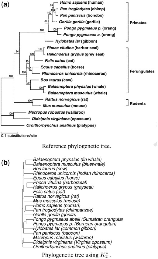
Reference phylogenetic tree from Cao et al. (1998), and the corresponding tree generated using the proposed $K_2^{*}$ alignment-free sequence comparison method, using the mtDNA20 dataset

Looking at these figures, we can see that the trees are generally similar to the reference tree, though with some variations. We can observe that $D_2$ and $D_2^{*}$ placed horse and white rhinoceros close to each other as expected, however, their parent nodes were wrongly placed, making them much further from say cow than in the reference tree. Also, $D_2$ wrongly placed wallaroo very close to mouse and rat, while $D_2^{*}$ had cow much closer to rat and mouse than the reference tree. $D_2^{sh}$ provided a better result than $D_2$ and $D_2^{*}$⁠, but it also incorrectly placed platypus much closer to rat and mouse. Methods $K_2$ and $K_2^{*}$ seem to avoid these problems. One quick way to access the performance of the methods is to compare the minimum number of hops needed to go from one given leaf node (representing a species) to another leaf node on a given tree. The Supplementary Table S3 shows the number of hops for two pairs of species. The Supplementary Figure S1 and Table S3 suggest that the proposed methods $K_2$ and $K_2^{*}$ work better than the other methods on the mtDNA20 dataset.

3.1.2 Fish23 dataset

Table 2 shows the Robinson-Foulds distances for the Fish23 dataset. Each column shows distances of one alignment-free method with parameter $k$ varied from 2 to 9. The last row shows the results for three methods that did not use varying $k$ parameters. The minimum distance in this table is $8$ (shown in boldface in the table). Methods $K_2^{*},\hspace{0.17em}{K}_2,\hspace{0.17em}{D}_2,\hspace{0.17em}{D}_2^{*}$ and $D_2^{sh}$ are able to achieve the minimum distance. As with the previous experiment on ‘mtDNA20’, $D_2^z,\hspace{0.17em}WFV,\hspace{0.17em}Shi$ and $DV$ are worse than the others. Among these methods, only $K_2^{*}$ is able to automatically determine an appropriate $k$ value. From these results, we conclude that with respect to phylogenetic trees, the $K_2^{*}$ is the best amongst all the tested alignment-free methods.

Table 2.

The Robinson-Foulds distance between the reference phylogenetic tree and phylogenetic trees generated using different alignment-free statistical methods (with $k=2,3,\dots 9$⁠)

k	$D_2$	$D_2^{*}$	$D_2^{sh}$	$D_2^z$	$K_2$	$DMk$	$CPF$	$WFV$
2	32	34	36	40	36	30	32	36
3	30	30	28	40	26	28	30	30
4	26	26	30	36	24	22	24	26
5	24	20	22	38	20	20	20	26
6	14	10	20	36	12	10	12	32
7	14	8	14	34	8	12	12	34
8	8	8	8	34	8	12	14	34
9	8	10	14	—	10	14	16	34
	$K_2^{*}$	8		$DV$	32		$Shi$	34

Note: Results are based on the Fish23 dataset (Fischer et al., 2013). For brevity, the results for $K_2^{*}$ (with automatically determined $k$ value), and DV and Shi (both with fixed $k$ parameters), are reported in the last row. $D_2^z$ generated an error at $k=9$⁠. The bold value 8 here indicates the minimal RF distance. The smaller the RF distance is, the better a method performs.

The Supplementary Figure S2a shows the phylogenetic tree reported by Fischer et al. (2013) in their original paper using the Fish23 dataset. Similar to the ‘mtDNA20’ experiment, we show the phylogenetic trees generated by the alignment-free methods: $D_2,\hspace{0.17em}{D}_2^{*},\hspace{0.17em}{D}_2^{sh}$⁠, $DMk,\hspace{0.17em}CPF$⁠, $K_2$ and $K_2^{*}$⁠. The Supplementary Figure S2(b–h) show the phylogenetic trees with the minimum Robinson-Foulds distance for each method. Supplementary Figure S2a is the reference tree. For our experiments, since we did not have the sequences for P.trewavasae and T.moorii, the pairs N.brichardi, T.duboisi will become neighbors, with parent at node 16 in the original reference tree.

Fish Dataset demonstrates similar trends to the mtDNA20 dataset, see more details in Supplementary Material, Section 4.3.

3.2 Correlation with the edit distance

3.2.1 mtDNA20 dataset

Table 3 shows the Pearson correlation coefficients between the similarity measurements from the different alignment-free methods and the edit distance, using the mtDNA20 dataset. From the table, one can observe that $D_2^{sh}$ achieved the best result $-0.92$ when $k=6$ or $k=7.K_2$ achieve the best result (⁠$\rho =-0.95$⁠) when $k=9.K_2^{*}$ can reach $\rho =-0.94$ which is close to the best of $K_2$⁠. In a word, the $K_2$ method can reach the best accuracy, and $K_2^{*}$ is quite competitive. A key advantage of the $K_2^{*}$ method is that it is able to select parameter $k$ automatically and quickly. However, considering the $K_2$ may need to try all possible $k$ values to determine the best $k$ (9 in this case), the slight performance disadvantage (⁠$\rho =0.94$ versus $\rho =0.95$⁠) of $K_2^{*}$ becomes even less significant, especially when data volume is huge. See more detailed analysis in Supplementary Material, Section 4.1.1.

Table 3.

Pearson correlation coefficient between the similarity/distance measure from different alignment-free statistical methods and the edit distance

k	$D_2$	$D_2^{*}$	$D_2^{sh}$	$D_2^z$	$K_2$	$DMk$	$CPF$	$WFV$
2	−0.45	−0.51	−0.55	0.02	−0.56	0.67	0.62	0.57
3	−0.48	−0.60	−0.74	0.10	−0.73	0.68	0.66	0.62
4	−0.53	−0.71	−0.86	−0.74	−0.82	0.70	0.71	0.63
5	−0.61	−0.79	−0.91	−0.81	−0.89	0.78	0.77	0.72
6	−0.77	−0.87	−0.92	−0.83	−0.92	0.84	0.86	0.68
7	−0.87	−0.91	−0.92	−0.84	−0.92	0.87	0.89	0.68
8	−0.90	−0.92	−0.91	−0.84	−0.93	0.85	0.89	0.66
9	−0.91	−0.91	−0.91	—	−0.95	0.85	0.87	0.67
	$K_2^{*}$	−0.94		$DV$	0.70		$Shi$	0.68

Note: Reports are for the mtDNA20 dataset. $K_2^{*}$ having automatically determined $k$ values, $DV$ and $Shi$ without varied $k$ parameter, they are all reported in the last row for brevity. $D_2^z$ generated an error at $k=9$⁠. The bold values indicate the biggest absolute value of Pearson correlation coefficient for different k values. The bigger an absolute value, the better a method performs.

Similar results were observed using the Fish23 dataset. These have been included in Section 4.1.2 of Supplementary Material.

3.3 Practical running time

We compare the running time of eleven methods, [9 earlier approaches (⁠$D_2,\hspace{0.17em}{D}_2^{*},\hspace{0.17em}{D}_2^{sh},\hspace{0.17em}{D}_2^z,\hspace{0.17em}DMk,\hspace{0.17em}CPF,\hspace{0.17em}WFV,\hspace{0.17em}DV$ and $Shi$⁠) and the two proposed methods (⁠$K_2$ and $K_2^{*}$⁠)].

3.3.1 mtDNA20 dataset

Table 4 shows a comparison of the running time for eleven methods using the first dataset (mtDNA20 dataset) from Cao et al. (1998). Figure 2 plots the corresponding running times. The time for $K_2^{*}$ is 3.07 s, time for $DV$=2.33 s and time for $Shi$=1.37 s which are not plotted in the figure. When $k=9,\hspace{0.17em}{D}_2^z$ generates a runtime error, thus, we could not obtain a result for this case.

Table 4.

Practical running time (in seconds) using alignment-free methods on the mtDNA20 dataset

$k$	$D_2$	$D_2^{*}$	$D_2^{sh}$	$D_2^z$	$K_2$	$DMk$	$CPF$	$WFV$
2	0.02	0.05	0.05	1.55	0.41	3.64	13.23	0.004
3	0.03	0.05	0.07	1.56	0.45	4.90	14.02	0.008
4	0.08	0.11	0.15	1.61	0.57	5.91	15.63	0.020
5	0.20	0.34	0.5	1.76	1.94	7.06	16.82	0.088
6	0.56	1.29	2	2.35	2.22	9.78	16.58	0.884
7	1.26	4.91	7	5.38	3.17	18.09	16.43	7.768
8	2.40	18.18	25	19.19	3.63	40.13	16.82	38.3
9	4.58	70.28	99	—	4.34	92.10	17.05	347.1
	$K_2^{*}$	3.07		$DV$	2.33		$Shi$	1.37

Note: Results for $K_2^{*}$ with automatically determined $k$ values, $DV$ and $Shi$ with fixed $k$ values, are reported in the last row. $D_2^z$ generated an error at $k=9$⁠. The bold values shown the smallest running time (the fastest method) for different k values.

Fig. 2.

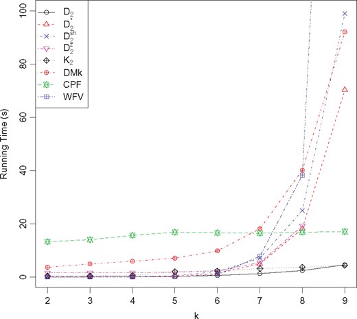
Time cost comparison for $D_2,\hspace{0.17em}{D}_2^{*},\hspace{0.17em}{D}_2^{sh},\hspace{0.17em}{D}_2^z,\hspace{0.17em}DMk,\hspace{0.17em}CPF,\hspace{0.17em}WFV$ and $K_2$ with parameter $k$ varying from 2 to 9, using the mtDNA20 dataset. Results for $K_2^{*}$=3.07 s, $DV$=2.33 s and $Shi$=1.37 s are not shown in the figure for clarity

First, consider the methods that use varied $k$ values. When $k<6$⁠, the $WFV$ approach is the fastest among all methods. When the parameter $k$ increases, the running time of $WFV$ increases rapidly, much quicker than all the others. When $k=7,8,9,\hspace{0.17em}WFV$ requires approximately 2.45, 10.55 and 109.5-fold time increases, respectively, when compared with $K_2$⁠. Therefore, in terms of running time, $K_2$ is the better choice than the other methods, with less running time and higher accuracy when $k>6$⁠. The $WFV$ method with RF distances (26, 24 and 22) shown in Table 1 did not perform well.

Consider $D_2^{sh}$ and $K_2$⁠, the two methods that achieved the best results with RF distance = 12 in Table 1. $D_2^{sh}$ reaches its best performance when $k=7,8.K_2$ reaches its best performance when $k=8,9$⁠. When $k=7,8,9,\hspace{0.17em}{D}_2^{sh}$ requires approximately 2, 8 and 25 fold time increases, respectively, when compared with $K_2$⁠. Therefore, in terms of combining with running time and accuracy, $K_2$ is the better choice than $D_2^{sh}$⁠.

Now consider $K_2^{*},\hspace{0.17em}DV$ and $Shi$ which do not use varying $k$ values. $K_2^{*}$ requires 3.07 s to execute. $DV$ and $Shi$ are relatively faster with 2.33 and 1.37 s respectively. However, $K_2^{*}$ generated a much lower RF distance—see Table 1. $K_2^{*}$ is slower than the other methods (i.e. $D_2,\hspace{0.17em}{D}_2^{*},\hspace{0.17em}{D}_2^{sh}$⁠) with $k=2,3,4,5,6$⁠, and faster than the other methods with $k=7,8,9$⁠. We can also observe from the results discussed earlier that, for this dataset, the best performance for the other methods were recorded at k ≥ 6. See Supplementary Figure S1 and Table 1. Clearly, since $K_2^{*}$ does not need to search for the best $k$ value (i.e. it is executed for just one $k$ value), it is overall faster than the other methods, without degrading the accuracy. This is important, considering the increasingly huge volumes of data involved in most applications of these techniques. In fact, the primary motivation for the alignment-free methods is their rapid processing speed, when compared with alignment-based methods.

Results on running time using the Fish23 dataset is provided in the Supplementary Material.

With respect to running time, we can identify two key points from our experiments: (i) the running time for $D_2^{sh},\hspace{0.17em}{D}_2^z$⁠, $DMk$ and $WFV$ increases rapidly with increasing $k$⁠. The running time for $K_2$ is approximately linear with respect to the sequence length. (ii) Comparing $K_2$ and $K_2^{*},\hspace{0.17em}{K}_2^{*}$ is more practical, since it can determine the $k$ value automatically, and has a competitive performance.

3.4 Evaluation on functionally related regulatory sequences

While the alignment-free methods could be generally fast, an important consideration is whether they can identify similarities between sequences that are functionally related. Of course, this can only be possible if the sequences share some similar patterns. To evaluate this aspect of performance, we consider to what extent the alignment-free similarity measures are able to capture the similarities between sequences from the same anatomic regions of the same species. For this experiment, we used the third dataset—CRM185 dataset, the regulatory sequences from Kantorovitz et al. (2007). We compare our proposed methods $K_2$ and $K_2^{*}$ against $D_2^z,\hspace{0.17em}{D}_2,\hspace{0.17em}{D}_2^{sh}$ and $D_2^{*}$⁠, $DMk,\hspace{0.17em}DV,\hspace{0.17em}CPF,\hspace{0.17em}Shi$ and $WFV$⁠. Table 5 shows the results. In the table, the result for $D_2^z$ is taken from the original work of Kantorovitz et al. (2007). For $D_2^z,\hspace{0.17em}{D}_2,\hspace{0.17em}{D}_2^{sh}$ and $D_2^{*}$⁠, the table shows the best results with $k$ values in the range $2\le k\le 7$⁠. For $K_2$ method, we also tested with $2\le k\le 7$⁠.

Table 5.

The performance of popular alignment-free sequence similarity methods in capturing functional relatedness

Species	Dataset	$D_2^z$	$K_2$	$D_2$	$D_2^{sh}$	$D_2^{*}$	$K_2^{*}$	$DMk$	$CPF$	$WFV$	$DV$	$Shi$
Fly	Blastoderm	0.73	0.92(4)	0.85(2)	0.82(2)	0.82(6)	0.79	0.83(3)	0.84(4)	0.79(5)	0.72	0.7
Fly	PNS	0.62	0.60(5)	0.63(3)	0.64(4)	0.64(3)	0.56	0.62(4)	0.61(4)	0.63(3)	0.58	0.55
Fly	Tracheal	0.75	0.75(4)	0.72(4)	0.69(4)	0.69(4)	0.75	0.73(3)	0.75(4)	0.70(5)	0.7	0.71
Fly	Eye	0.58	0.69(3)	0.61(2)	0.63(3)	0.60(3)	0.69	0.63(5)	0.63(4)	0.64(3)	0.62	0.59
Human	Muscle	0.83	0.88(4)	0.83(5)	0.83(5)	0.86(6)	0.81	0.84(3)	0.82(4)	0.81(5)	0.76	0.79
Human	Liver	0.69	0.83(2)	0.88(2)	0.78(6)	0.73(4)	0.69	0.82(2)	0.84(5)	0.80(3)	0.8	0.76
Human	HBB	0.64	0.65(3)	0.58(3)	0.53(2)	0.59(4)	0.66	0.57(2)	0.60(3)	0.61(4)	0.56	0.52

Note: Numbers in brackets indicate the $k$ value that produced the best results for the given method. Results are based on the CRM185 dataset. The bold values shown the best methods on a data set without considering K₂* and with considering K₂*.

The bold items are the best results on the dataset comparing different methods, while excluding $K_2^{*}$⁠. From Table 5, $K_2$ reported five best results out of seven using the CRM185 dataset. $D_2^z,\hspace{0.17em}{D}_2,\hspace{0.17em}{D}_2^{sh}$ and $D_2^{*}$ reported one best result each. $K_2$ demonstrates competitive performance with the other methods. When we take $K_2^{*}$ into consideration, we can observe that it gets three best results out of seven datasets. $D_2^z$ and $D_2^{sh}$ get one best result of seven cases, $D_2^{*}$ and $D_2$ are best on two cases, and $K_2$ was best on four cases. In general, the proposed $K_2$ and $K_2^{*}$ methods provide the overall best performance on this problem.

4 Conclusion

The problem of sequence similarity measurement is critical to several important applications in huge volume genomic sequence analysis. We proposed a novel non-parametric algorithm $K_2$ for alignment-free measurement of relatedness between sequences, using the statistics of $k$-grams in the sequences. $K_2$ is a non-parametric approach based on the Kendall correlation statistic to estimate the dissimilarity(/similarity) of sequences.

Compared with other state-of-the-art alignment-free comparison methods (⁠$D_2,\hspace{0.17em}{D}_2^{*},\hspace{0.17em}{D}_2^{sh},\hspace{0.17em}{D}_2^z,\hspace{0.17em}DMk,\hspace{0.17em}CPF,\hspace{0.17em}WFV,\hspace{0.17em}DV$ and $Shi$⁠), $K_2$ demonstrates comparable or better performance, in phylogenetic analysis, in generating (similarity/dissimilarity) measures that correlate with the edit distance among a large number of sequences, and in capturing functional relatedness between sequences. Further, the $K_2$ approach is faster than the other methods when $k\ge 7.$

We also introduced $K_2^{*}$⁠, an improved version of $K_2$ that is able to automatically determine the suitable $k$ value, thus eliminating the need to search for all possible $k$ values (for the $k$-grams), potentially from $k=2$ to $k=n\hspace{0.17em}.K_2^{*}$ produced the best overall results, with respect to both efficiency and accuracy. Along with $K_2^{*}$ competitive performance in measuring the similarity between sequences, its speed makes it practical, an important consideration given the increasingly huge datasets in various applications of alignment-free methods.

Acknowledgement

A shorter version of this paper was presented at IEEE BIBM’2016, Lin et al. (2016).

Funding

This work was supported by the Chinese National Natural Science Foundation (Grant No. 61472082), Natural Science Foundation of Fujian Province of China (Grant No. 2014J01220), the US National Science Foundation (Grant No. IIS-1552860) and Scientific Research Innovation Team Construction Program of Fujian Normal University (Grant No. IRTL1702).

Conflict of Interest: none declared.