Ontological function annotation of long non-coding RNAs through hierarchical multi-label classification

Abstract

Motivation

Long non-coding RNAs (lncRNAs) are an enormous collection of functional non-coding RNAs. Over the past decades, a large number of novel lncRNA genes have been identified. However, most of the lncRNAs remain function uncharacterized at present. Computational approaches provide a new insight to understand the potential functional implications of lncRNAs.

Results

Considering that each lncRNA may have multiple functions and a function may be further specialized into sub-functions, here we describe NeuraNetL2GO, a computational ontological function prediction approach for lncRNAs using hierarchical multi-label classification strategy based on multiple neural networks. The neural networks are incrementally trained level by level, each performing the prediction of gene ontology (GO) terms belonging to a given level. In NeuraNetL2GO, we use topological features of the lncRNA similarity network as the input of the neural networks and employ the output results to annotate the lncRNAs. We show that NeuraNetL2GO achieves the best performance and the overall advantage in maximum F-measure and coverage on the manually annotated lncRNA2GO-55 dataset compared to other state-of-the-art methods.

Availability and implementation

The source code and data are available at http://denglab.org/NeuraNetL2GO/.

Supplementary information

Supplementary data are available at Bioinformatics online.

1 Introduction

Long non-coding RNAs (lncRNAs), which have little or no potential to encode for functional proteins (Mercer et al., 2009), have a wide distribution in organisms. Large numbers of lncRNAs have been recognized in many organisms along with the development of DNA sequencing technologies. The number of lncRNAs increased significantly in recent years with the extensive utilization of experimental technologies to annotate transcriptome (Mortazavi et al., 2008). Large-scale analyses of the transcriptome have revealed that the types and number of lncRNAs are far more than those of protein-coding transcripts (Birney et al., 2007). Accumulating evidence shows that lncRNAs are involved in many biological processes, such as immune response, development, differentiation and gene imprinting (Morris and Mattick, 2014; Tang et al., 2016; Turner et al., 2014) and are associated with diseases and cancers (Wapinski and Chang, 2011; Zhang et al., 2017; Zou et al., 2015a, b). However, the functions of most lncRNAs and the underlying molecular mechanisms of gene regulation remain unclear. Hence, the annotation of lncRNA functions has become an area of focus in the fields of biology and bioinformatics.

Currently, some biological schemes for determining the functions of lncRNAs are as follows: analysis of lncRNA high-throughput expression profiles (Liu et al., 2017), verification of high-throughput data and exploring lncRNA function as part of interactions. The high-throughput analysis of lncRNA expression profiles is performed through microarrays and RNA-seq (Mortazavi et al., 2008). Li et al. (2016) utilized quantitative RT-PCR to detect the expression profiles of lncRNA TUG1 in glioma tissues and conducted correlation analysis to reveal the relationship between TUG1 expression and different clinicopathologic parameters. They also researched into the function and found the influence of TUG1 on apoptosis and cell proliferation. In addition to expression-based methods, the application of next-generation sequencing technology opens up a new way for us to construct genome-wide interaction maps for biomolecules (Garzón et al., 2016). The biological function of lncRNAs in the cell could be considered as a function of biological interactions mediated by lncRNAs with other biomolecules (e.g. DNAs, RNAs, proteins). Some well-characterized lncRNAs (e.g. HOTTIP, HOTAIR) carry out their function by interacting with DNA (Mercer and Mattick, 2013). Many experimental methods to investigate RNA–DNA interactions have been proposed in recent years, such as chromatin isolation by RNA purification developed by Jeffrey and his cooperators (Jeffrey and Chang, 2012) and capture hybridization analysis of RNA targets designed by Simon (2013). Apart from interaction with DNA, lncRNAs have been demonstrated to interact with RNAs. Among various types of RNA, interactions with miRNA are most well-studied (Paraskevopoulou and Hatzigeorgiou, 2016), for example, lncRNA could act as a sponge to regulate the behavior of regulatory miRNAs (Ebert and Sharp, 2010). Besides with DNA and RNA, interactions with protein are pervasive and protein–RNA interactions are crucial aspects of many cellular processes (Yu et al., 2017). Ferrè et al. addressed the approaches to reveal the lncRNA–protein interactions (Ferrè et al., 2016). To explore the function of lncRNAs, it is usually necessary to combine one or more of the above-described interactions.

The experimentally identifying functions of lncRNAs are usually expensive and progressing slowly. Computational methods for predicting lncRNA function become more and more important. Since genes with identical or similar functions tend to have similar expression patterns across multiple different tissues (Lee et al., 2004), it is an efficient approach to analyze the role of the lncRNAs by analyzing the co-expression patterns shared with their neighboring counterparts (Necsulea et al., 2014). Guttman et al. (2009) identified some lincRNAs, then computed functional associations using gene set enrichment analysis (GSEA). GSEA was based on co-expression patterns, but the authors did not build a complete co-expression network. In another study, the researchers constructed a coding and non-coding gene co-expression network according to the abundant expression profiles in the GEO database, then predicted the functions of more than 300 mouse lncRNAs based on co-expression and genomic co-location (Qi et al., 2011). Guo et al. (2013) developed an approach named lnc-GFP to predict function for 1625 lncRNAs. In lnc-GFP, a bi-colored biological network was constructed and took into account both coding and non-coding co-expression profiles and protein–protein interactions. In 2015, Jiang et al. (2015) computed the Pearson correlation coefficients (PCCs) of all lncRNA-mRNA gene pairs according to the expressions of all human lncRNAs and mRNAs in the 19 tissues and then annotated 9625 human lncRNAs by employing the hypergeometric test.

In this work, we propose NeuraNetL2GO, which uses multiple neural networks to annotate probable function of lncRNAs at a large scale (Cerri et al., 2014; Cerri et al., 2015; Ricardo et al., 2016). First, we construct a lncRNA-lncRNA biological network according to lncRNA co-expression data. Second, we generate the topological feature vectors of the co-expression network by running random walks with restart (RWR; Tong et al., 2006). Finally, we build multiple neural networks, in which the topological feature vectors are used as inputs, and the gene ontology (GO) terms are the output labels of these neural networks. We generate 13 neural networks in total since the GO terms are distributed over the 13 levels in the directed acyclic graph (DAG) hierarchy of GO and each neural network corresponds to the GO terms in one level. In the independent test, we achieve a maximum F-measure of 0.336 on the manually annotated 55 lncRNAs with 129 GO terms, which is significantly better than that of the other two state-of-the-art methods: lnc-GFP (Guo et al., 2013) and LncRNA2Function (Jiang et al., 2015).

2 Materials and methods

As an overview, the flowchart of our method is depicted in Figure 1. The primary processing is composed of several steps: (i) Construct the lncRNA similarity network according to the lncRNA expression profiles; (ii) diffusion component analysis (DCA) (Cho et al., 2015) is adopted to obtain a low-dimensional vector representation of each node in the lncRNA similarity network; (iii) Build the training GO annotation dataset using neighbor counting method (Wong and Chua, 2012); (iv) Train the multi-layer networks incrementally, level by level, and apply the neural networks to the independent test dataset and the human genome.

Fig. 1.

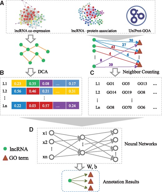
Flowchart of NeuraNetL2GO. It includes four steps: (A) Construct the lncRNA similarity network. (B) Extract topological features in the network with the DCA approach. (C) Build the training dataset by employing the Neighbor Counting method. (D) Training the multi-layer neural networks

2.1 Construct the lncRNA similarity network

The construction of the lncRNA similarity network is based on the assumption that transcripts which have similar expression patterns have similar functions or share related biological pathways. We calculate the PCC between the expression profiles of each pair of lncRNAs. The PCC values are used as the weights of the similarity networks.

2.2 Obtain a low-dimensional vector representation

In the lncRNA co-expression network, the nodes (lncRNAs) that are similar in the topological structure may have similar functions. We employ the DCA strategy to extract the low-dimensional topological information of lncRNAs. First, the RWR algorithm is performed on each node in the lncRNA similarity network. Since considering the local and global topological information in the network, RWR can select the relevant or similar nodes in the network.

Let $P_t$ be a vector in which the i-th entry holds the probability of the i-th node being visited at step t. The probability vector at step t + 1 can be decided by

$$p_{t+1}=(1-r)M^T{p}_t+r{p}_0.$$

(1)

The parameter r is the restart probability which is a balancing parameter determining the importance of local and global topological information; M is the transition probability of the network and $M^T$ is the transpose matrix of M. After a large number of steps, the probabilities will reach to a steady distribution which is called as the ‘diffusion state’. The steady probability provides a measurement of the proximity to the seed nodes. When the two nodes harbor similar diffusion states, it suggests that the two nodes are in similar positions in the network to other nodes. This means they are similar in function. However, the diffusion states are high-dimensional when the network is large and may have noise information. To solve this problem, we use singular value decomposition to reduce the dimensionality of diffusion states (Cho et al., 2015; Wang et al., 2015).

2.3 Build the training dataset

At present, the fact that there are no public GO annotations of lncRNAs limits the application of machine learning (Fan et al., 2016). Hence, we use the neighbor counting method to annotate some lncRNAs according to the known GO annotations of protein. This approach is based on the fact that the target lncRNA may have very similar functions as that of the direct neighbor proteins in the lncRNA-protein association network.

For each target lncRNA l in the lncRNA-protein association network, the frequency of appearance of each function $f_i\in F$ is calculated based on the direct neighbors of l, where F is the set of functions owned by all direct neighbors of l. The function is as follows:

$$S_f\left(L\right)={\sum }_{n\in N_l}I(n,f),$$

(2)

where $I(n,f)=1$ if the neighbor n has the function f, 0 otherwise. $N_l$ is the set of direct neighbors of lncRNA l in the lncRNA-protein association network. A proper minimum threshold frequency needs to be selected to adjust the prediction for lncRNA.

2.4 Train the multi-layer networks

Since GO functions are organized as a DAG hierarchy (Deng and Chen, 2015), the prediction of lncRNA functions can be considered as a hierarchical multi-label classification. We associate one neural network to each level of the class hierarchy. In this way, the complex learning model is split into simpler models. The multiple neural networks are trained sequentially, level by level. After the training process of one neural network for a certain level, both the predictions of the network and the feature information extracted from the instances belonging to the next level are employed to train the next neural network. The procedure keeps on until the last level.

The architecture of the multiple neural networks for a three-level hierarchy is illustrated in Figure 2. Here, $X_l$ is the feature vectors of the instances corresponding to classes from level l; $H_l$ and $O_l$ represent the hidden layer and output layer of the neural network at level l, respectively. The architecture of the neural network at each level includes one hidden layer and one output layer to be trained. In our work, the feature vectors of the instances are the low-dimensional vector-space representations for all nodes in the lncRNA similarity network. Since there are multiple GO terms at each level of the DAG hierarchy, each output neuron corresponds to one class, namely one GO term. First, the neural network corresponding to the first level 1 is trained (Fig. 2A), then the second neural network at level 2 follows. Besides the feature vectors of the instances that are assigned to the classes belonging to level 2 (⁠$X_2$⁠), the output of the neural network of level 1 is also the input of the network of level 2 (Fig. 2B). In the same way, the third neural network at level 3 is trained after the training of the neural network at level 2 is finished (Fig. 2C). The procedure of incremental training does not end until the neural network at the last level is trained. It should be pointed out that when a neural network at level l is trained, the neural networks at the previous levels are not re-trained since these networks have already been trained in the previous steps. The output of the network at level l – 1 only acts as a portion of the input for the network at level l. In our networks, we use the quadratic cost function and sigmoid function as the cost function and activation function, respectively. In training, the famous back-propagation is used to train the neural networks (Rumelhart et al., 1986). The pseudocodes for the training procedures are presented in Algorithm 1.

Fig. 2.

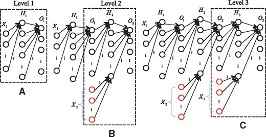
Architecture of the multiple neural networks for a three-level hierarchy. (A) Train a neural network for the first level. (B) Train a neural network for the second level, the input of which includes the features of the instances and the output of the neural network of level 1. (C) Use the output of the neural network of level 2 to augment the feature vectors for training the neural network of level 3

Algorithm 1

NeuralNETLGO algorithm

Require: X: feature matrix of training instances, y: label matrix of annotations, dataValid: feature matrix of validating instances, Levels: level number of the GO hierarchy, epochs: number of training epochs, η learning rate in Back-propagation, α: momentum factor in Back-propagation

Ensure: W: weights of the multiple neural networks

 //Initialize the weights of the multiple neural networks

 InitializeRandomWeights(W)

 fori = 1 to epochs

  forl = 1 to Levels

   forx in X

    //σ is activation function

    $a_1^{\mathrm{1}}=\sigma (W_1^{\mathrm{1}}{x}_1)$

    $a_2^{\mathrm{1}}=\sigma (W_2^{\mathrm{1}}{h}_1)$

    ifl = 1

     //Calculate error

     $err=y_1-a_2^{\mathrm{1}}$

     //Calculate gradients

     ${\delta }_2^{\mathrm{1}}=err\odot \sigma \prime (W_2^{\mathrm{1}}{h}_1)$

//Elementwise product

     ${\delta }_1^{\mathrm{1}}=({(W_2^{\mathrm{1}})}^T{\delta }_2^{\mathrm{1}})\odot \sigma \prime (W_1^{\mathrm{1}}{x}_1)$

     //Update weights

     $\Delta W_2^{\mathrm{1}}={\alpha }_2{(\Delta W_2^{\mathrm{1}})}^{i-1}+{\eta }_2({\delta }_2^{\mathrm{1}}\otimes a_1^{\mathrm{1}})$

     $\Delta W_1^{\mathrm{1}}={\alpha }_1{(\Delta W_1^{\mathrm{1}})}^{i-1}+{\eta }_1({\delta }_1^{\mathrm{1}}\otimes x_1)$

     $W_2^{\mathrm{1}}=W_2^{\mathrm{1}}+\Delta W_2^{\mathrm{1}}$

     $W_1^{\mathrm{1}}=W_1^{\mathrm{1}}+\Delta W_1^{\mathrm{1}}$

    else

     //Feedforward from level 2 to l

     forj = 2 to l

     $x_j=x_j\oplus a_2^{j-1}$ //Concatenate vectors

     $a_1^j=\sigma (W_1^j{x}_j)$

     $a_2^j=\sigma (W_2^j{a}_1^j)$

    end for

     $err=y_l-a_2^l$

     ${\delta }_2^l=err\odot \sigma \prime (W_2^l{h}_l)$

     ${\delta }_1^l=({(W_2^l)}^T{\delta }_2^l)\odot \sigma \prime (W_1^l{x}_l)$

     //Update weights in level l

     $\Delta W_2^l={\alpha }_2{(\Delta W_2^l)}^{i-1}+{\eta }_2({\delta }_2^l\otimes a_1^l)$

     $\Delta W_1^l={\alpha }_1{(\Delta W_1^l)}^{i-1}+{\eta }_1({\delta }_1^l\otimes x_l)$

     $W_2^l=W_2^l+\Delta W_2^l$

     $W_1^l=W_1^l+\Delta W_1^l$

    end if

   end for

  end for

  Measure = validate(W, dataValid)

  ifMeasure > bestMeasure

   bestMeasure= Measure

else

   earlyStop++

   ifearlyStop==maxEpochs

   break

  end if

 end if

end for

Return  W

We use a top-down strategy to predict the GO terms according to the test instances. The test examples act as the input for the neural network at the first level, and then the output from the first network, combining the feature vector of test example, is fed to the second neural network. The output values from the second network will augment the feature vector of test example belonging to the third level once again. The procedure is continued until the last network is reached. The output values for each level are achieved in sequence. When the procedure is finished, the output values of the output layers of the neural networks fall in the range [0, 1] since the sigmoid function is employed as activation function in the neurons. Different thresholds are applied to the output neurons of the networks to obtain the predicted GO terms for each level. If the output value of a neuron in the output layer is equal to or larger than a given threshold, the corresponding position of the class vector is set to 1. Otherwise, the position is assigned 0.

3 Results

3.1 Datasets and pre-processing

3.1.1 lncRNA co-expression similarity

We extract the lncRNA expression profiles from NONCODE2016 database (Xie et al., 2014), which provides the expression profiles of 90 062 lncRNAs in 24 human tissues or cell types. PCC between the expression profiles of each pair of lncRNAs is computed, and then the lncRNA similarity network is built according to the PCC scores between lncRNAs.

3.1.2 lncRNA-protein associations

The lncRNA-protein associations are computed based on the co-expression data and the interactions between lncRNAs and proteins. We downloaded all human lncRNA genes and protein-coding genes from the GENCODE Release 24 (Derrien et al., 2012) and extracted a total of 15 941 lncRNA genes and 20 284 protein-coding genes. Then, we calculated the co-expressions and interactions:

• Co-expression data from COXPRESdb (Okamura et al., 2015). We extracted three preprocessed co-expression datasets (Hsa.c4-1, Hsa2.c2-0 and Hsa3.c1-0) with pre-calculated pairwise PCC values for human from COXPRESdb. The correlations are calculated as follows:

  $$C_C(l,p)=1-\prod _{d=1}^D(1-C_d(l,p\left)\right)\hspace{1em}if\hspace{0.17em}{C}_d(l,p)>0,$$

  (3)

where C(l, p) is the overall correlation between gene l (lncRNA) and protein-coding gene p, $C_d(l,p)$ is the correlation score between l and p in dataset d, D is the number of pairs (l and p) with positive correlation scores.

• Co-expression data from ArrayExpress (Rocca-Serra et al., 2003) and GEO (Barrett et al., 2007). We obtained the co-expression data from the work of Jiang et al. (Jiang et al., 2015). PCC values (denoted as C_J) are used to evaluate the co-expression of lncRNA-protein pairs.

• LncRNA-protein interaction data. We extracted human lncRNA-protein interactions from Npinter 3.0 (Hao et al., 2016). The score I(l, p) is 1 if there exists an interaction between lncRNA l and protein p, otherwise the score is 0.

Finally, we computed overall association score for each lncRNA-protein pair by combining the three sources of co-expression and interactions:

$$A(l,p)=1-(1-C_C)(1-C_J)(1-I).$$

(4)

3.1.3 Benchmarks

The neural networks are trained using a predicted GOA-lncRNA dataset, which includes more than 4000 lncRNAs by employing the neighbor counting method according to the lncRNA–protein interactions. An lncRNA is annotated with a GO term if the number of protein neighbors annotated with the GO term is larger than a threshold N. In this paper, N is assigned 20. At last, a total of 4031 lncRNAs are annotated, 70% of which are randomly chosen as the training data (2821 lncRNAs) and the rest are used as validation data (1210 lncRNAs). In our method, each class needs to be defined to a definite level. However, in DAG structures, which level a class belongs to is determined by the hierarchical path chosen from the root node to the class. In our method, the longest path (the deepest hierarchy) from the class to the root node is treated as the level of a class in the DAG structure. In this way, when a class is defined to a level l, all its superclasses will be defined to levels shallower than l.

Since there is no available public database of lncRNA function annotations, we manually curate a independent test set of 55 lncRNAs with 129 GO terms (lncRNA2GO-55) based on references. The lncRNA2GO-55 dataset only includes lncNRAs that have been functionally characterized through knockdown or over-expression experiments.

3.2 Evaluation measures

The output of our method for each term in the GO is a score in the interval [0, 1]. Hence, a threshold value is applied to determine the final predictions. For a given example, if the output for a class is equal to or greater than the threshold, the example is considered to belong to the class, otherwise it is not. We use t to denote the threshold value, P(t) to denote the set of predicted terms, and T to denote a set of experimentally determined GO terms. TP, FP and FN represent the number of true positives, false positives, and false negatives, respectively. For each lncRNA i and threshold t, they are given by

$$T{P}_i={\sum }_{f\in O}I(f\in P_i(t)\wedge f\in T_i)$$

(5)

$$F{P}_i={\sum }_{f\in O}I(f\in P_i(t)\wedge f\notin T_i)$$

(6)

$$F{N}_i={\sum }_{f\in O}I(f\in T_i\wedge f\notin P_i(t\left)\right).$$

(7)

Here, f is a GO term and O is the set of GO terms in our experiment. Function I(x) is an indicator function defined as:

$$I\left(x\right)=\{\begin{array}{c}1\\ 0\end{array} \begin{array}{c}x=\text{true}\\ x=\text{false}.\end{array}$$

(8)

For a given threshold t, the overall precision and recall for all example are defined as:

$$\text{Prec}=\frac{{\sum }_{i}T{P}_i}{{\sum }_{i}T{P}_i+{\sum }_{i}F{P}_i}$$

(9)

$$\text{Rec}=\frac{{\sum }_{i}T{P}_i}{{\sum }_{i}T{P}_i+{\sum }_{i}F{N}_i}$$

(10)

Low threshold engenders each example having many GO terms and brings about high recall and low precision. On the other hand, large threshold engenders few GO terms being assigned to each example and brings about high precision and low recall. To cope with the problem and provide a single-score for overall evaluation of different methods, the maximum F-measure over all thresholds (all points in the precision-recall curve) is calculated. The F_max is written as:

$$F_{\text{max}}=\underset{t}{\text{max}}\left(\frac{2·\text{Prec}\left(t\right)·\text{Rec}\left(t\right)}{\text{Prec}\left(t\right)+\text{Rec}\left(t\right)}\right).$$

(11)

Also, coverage is used to evaluate our method and compare it with other methods. It is defined as the ratio of the portion of lncRNAs annotated with GO annotations to the whole number lncRNAs.

3.3 Post processing

In NeuraNetL2GO, each neural network gives the predictions for the examples at each level. Namely, the prediction value in a level is not determined by the output of the neural network at other levels. Hence, classification inconsistencies may occur in terms of the predictions, i.e. when a subclass is predicted but its superclass is not. Figure 3 shows an example of the classification inconsistencies. Figure 3A illustrates a small part of the GO hierarchy taxonomy. The digits in the circles are the indices of the class in our experiment. The GO terms next to the circles correspond to the indices, respectively. The vector of prediction values is shown in Figure 3B, and the vector of predicted classes is obtained after a threshold value of 0.5 is used (Fig. 3C). The class corresponding to 196 is assigned 1(the red), but its superclass corresponding to 73 is assigned 0. The case is considered to be an inconsistency. Therefore, the value of the position is corrected to 0 (Fig. 3D).

Fig. 3.

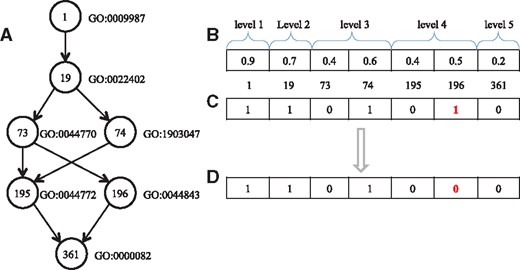
Example of the classification inconsistencies. (A) an example of the GO hierarchy. (B) the vector of predicted values. (C) the binary vector of predicted classes when a threshold value of 0.5 is used. (D) the binary vector of predicted classes after post processing

Another post-processing step needs to be highlighted. In DAG, there may be multiple paths from an ancestor to one descendant node, i.e. there are three paths from the node with index 1 to the node with index 361 in Figure 3A. The three paths are 1->19->73->195->361, 1->19->74->195->361 and 1->19->73->196->361. If there is one path that has been correctly predicted, all the superclasses will be set to 1. For example, if 1->19->73->195->361 is correctly predicted, the superclasses of node with index 361, namely, all the nodes in Figure 3A, will be assigned 1.

3.4 Parameter selection

There are many hyper parameters to be optimized, and parameter optimization is a complicated problem to solve. The hyper parameters utilized in our method are selected without exhaustive experiments. The hyper parameters to be optimized are as follows:

• Number of hidden neurons in each neural network. There are 13 neural networks in all, each corresponding to one level of the GO hierarchy.

• Momentum factor and learning rate used in Back-propagation with momentum algorithm.

• Initializations for the weights and biases in the neural networks.

• Number of lncRNA features (N_feature), namely, the number of dimensions of low-dimensional vector representation of each node in the lncRNA similarity network.

• The threshold N_neighbor used to determine if a lncRNA has the function of a GO term (the number of neighbors in the lncRNA–protein interactions corresponding to a GO term).

The first three categories of hyper parameters are used in the neural networks. We utilize the same values as Cerri et al.’s research (Cerri et al., 2015). As the depth of the hierarchy in DAG becomes deep, the training samples are gradually reduced. Therefore, to reduce overfitting, we gradually decrease the number of hidden neurons as the level is getting deeper. The number of hidden neurons is determined by setting the ratio of them to the number of neurons in input layer. These ratios are as follows: 0.65/0.65/0.6/0.55/0.5/0.45/0.4/0.35/0.3/0.25/0.2/0.15/0.1. The learning rate and momentum factor utilized in Back-propagation for hidden layers and output layers are 0.05, 0.03 and 0.03, 0.01, respectively. The initial values of the weights and biases in the neural networks in our experiment are selected randomly from the range [−0.1, 0.1].

Besides the hyper-parameters related to neural networks, the number of lncRNA features (N_feature) and the threshold N_neighbor also have significant influence on the prediction performance. In order to evaluate the impact of the two hyper-parameters on the functional annotations of lncRNAs, we vary their values and perform the independent test using the lncRNA2GO-55 dataset. Table 1 shows the comparison of the F_max when the two hyper-parameters are assigned different values. It can be observed that the F_max value reaches the max value when the number of lncRNA features (N_feature) and the threshold N_neighbor are set to 50 and 20, respectively. Hence, the two parameters, N_feature and N_feature, are set to 50 and 20, respectively, in this work.

Table 1.

The F_max values when using different combinations of the two hyper-parameters

Nneighbor	Nfeature
	50	100	200
10	0.1455	0.1458	0.1841
20	0.3361	0.2799	0.2309

3.5 Performance

As described earlier, the computational methods that investigate the functions of lncRNAs are mainly based on ‘guilt-by-association’ from co-expression patterns shared with their protein-coding counterparts. Among these methods, Liao et al.’s module-based method is based on a local strategy and only 340 lncRNAs have been functionally characterized (Qi et al., 2011). Lnc-GFP (Guo et al., 2013) is an important method that can annotate probable functions for lncRNAs on a large scale. In Lnc-GFP, a coding-non-coding bi-colored biological network is constructed according to gene expression data and protein–protein interaction data. Then a global propagation algorithm on the bi-colored network is used to predict putative functions for lncRNAs based on the known functions of proteins. LncRNA2Function (Jiang et al., 2015) is a method based on statistics. In LncRNA2Function, the hypergeometric test is employed to infer the functions of lncRNAs of interest according to the expression correlation between lncRNAs and protein-coding genes across 19 human normal tissues. Our NeuraNetL2GO approach is based on machine learning. We constructed multiple neural networks to predict probable functions for all the lncRNAs characterized in the lncRNA co-expression network.

In order to examine our method level by level, we calculated the maximum F-measure when predicting function classes of lncRNAs in different hierarchical levels. As shown in Figure 4, the performance of level 1 is the best and the maximum F-measure is 0.745. As the depth of the hierarchy increases, the performance gradually deteriorates. In GO hierarchy, the parent terms are more generalized and the child terms are more specific.

Fig. 4.

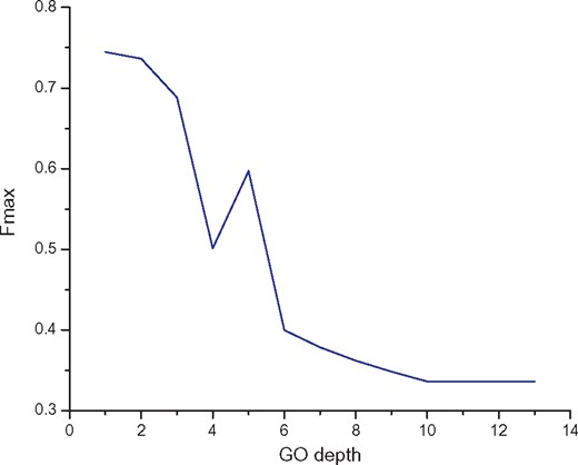
Performance comparison of different levels in the GO hierarchy

In this paper, we compare the performance of our method with the two state-of-the-art methods (lnc-GFP and LncRNA2Function) on the lncRNA2GO-55 dataset by an independent test. The GO classifies functions on three aspects: molecular function, cellular component and biological process. In our experiment, we compare the biological process with the other two methods since many lncRNAs participate in the biological process by lncRNA–protein interactions and most annotations in lncRNA2GO-55 are biological process terms. Performance comparison of the three methods is shown in Figure 5. Our NeuraNetL2GO method shows a much better performance in terms of maximum F-measure of 0.336, and lnc-GFP and LncRNA2Function follow with the maximum F-measure of 0.225 and 0.161. In precision and recall, our method also gains competitive scores of 0.250 and 0.513, respectively. Also, we calculate the numbers of lncRNAs that are annotated with at least one biological process GO term (excluding the root GO: 0008150) by the three methods. As shown in Figure 6, 50 lncRNAs are annotated correctly by our method. The coverage of NeuraNetL2GO is much higher than that of lnc-GFP and LncRAN2Function.

Fig. 5.

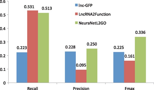
Performance comparison with the methods of lnc-GFP and LncRNA2Function

Fig. 6.

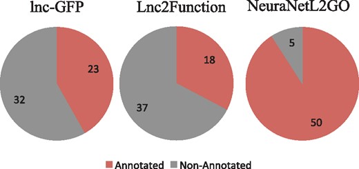
The numbers of lncRNAs that are annotated correctly by the three methods, respectively

3.6 Case studies

In this section, two lncRNAs are used as instances to further demonstrate the predictive performance and show the application of our method. For each lncRNA, the predicted GO terms, GO names and GO paths are listed in Supplementary tables.

Case study 1: HOTAIRM1. HOTAIRM1 is an lncRNA located between the HOXA1 and HOXA2 genes in humans, and it is transcribed antisense by RNA polymerase II. Researchers have demonstrated that HOTAIRM1 may play a regulatory role in myeloid transcriptional regulation and quantitatively impairs expression of the genes HOXA1 and HOXA4 (Zhang et al., 2009). Marina et al. (2015) found that HOTAIRM1 plays a role in normal hematopoiesis and leukemogenesis, including miR-196 b. The current studies have revealed that members of the integrin families take part in phagocytosis, leukocyte trafficking and signal transduction and are regulated by HOX genes (Dupuy and Caron, 2008). Also, HOTAIRM1 regulates genes encoding cell adhesion receptors. Zhang et al. (2014) revealed that E2Fs, HOTAIRM1 and perhaps protein-coding HOX genes might serve as a network to regulate cell cycle progression during differentiation. And their results suggest that an HOTAIRM1-regulated integrin switch mechanism involving CD11c and CD49d may regulate the cell growth in NB4 acute promyelocytic leukemia cells and hence modulate NB4 cell maturation.

We use NeuraNetL2GO to predict the functions of HOTAIRM1. The GO terms assigned to the lncRNA HOTAIRM1 are shown in Supplementary Table S1. Most of them are related to biological regulation, signal transduction and cellular process. These functions have been demonstrated by the previous studies. The results show that NeuraNetL2GO can successfully infer the functions of lncRNA HOTAIRM1.

Case study 2: GAS5. GAS5 (growth arrest-specific transcript 5) was originally identified from NIH3T3 cells using subtraction hybridization (Schneider et al., 1988). There exist many different patterns of alternative splicing in GAS5 transcripts. The open reading frame in GAS5 exons is small and poorly conserved during even relatively short periods of evolution (Schneider et al., 1988; Raho et al., 2000). Some studies have shown that GAS5 is related to apoptosis and it could play a role in the progression of numerous human cancers. For example, GAS5 has been shown to be a key regulator of prostate cell survival, and its levels in cellular are quantitatively related to cell death (Pickard et al., 2013). Mazar et al. (2017) found multiple novel splice variants by further analysis of sequenced GAS5 clones, the two variants of which were called Full-Length (FL) and Clone 2 (C2). The FL variant further promoted cell proliferation by rescuing cell cycle arrest, while the C2 variant had only a minimal effect on apoptosis. They also demonstrated that GAS5 expression has a significant impact on neuroblastoma cell biology.

To further assess the performance, we run NeuraNetL2GO on the lncRNA GAS5 according to the trained parameters. The GO terms predicted are listed in Supplementary Table S2. As expected, some of them are the apoptotic process, some regulation of cellular process, some cell cycle and so on. These predicted functions of GAS5 are consistent with the experimental results described earlier.

4 Discussion and conclusion

A huge number of lncRNAs have been recognized in the past few years. However, most of the lncRNAs remain poorly functional characterized. In this study, we propose a hierarchical multi-label classification strategy to annotate the functions of lncRNAs. First, we constructed an lncRNA similarity network according to the lncRNA expression profiles and extracted a low-dimensional vector representation of each node by running RWR on the network. Then multiple neural networks are trained with the low-dimensional vector representations as features of inputs and GO terms as outputs. After training these neural networks, the lncRNA2GO-55 dataset is employed to evaluate the performance independently. Regarding the experimental results, our NeuraNetL2GO method achieves the best prediction results, when compared to the other two state-of-the-art methods: lnc-GFP and LncRNA2Function. Moreover, 50 of the manually annotated 55 are correctly annotated with at least one GO term, which overwhelmingly outperforms the other two methods.

We would like to point out that our NeuraNetL2GO method may have some limitations. First, we have to employ the neighbor counting method to annotate some lncRNAs to train the neural networks because of the lack of experimentally determined lncRNA function annotations. It would lead to a bias against the correct annotations. Second, low-dimensional vector representation of each node is extracted depending on the structure of lncRNA similarity network. However, low-dimensional vector representation of each node is inexact since the expressions of many lncRNAs are missing. Third, it is challenging to set so many hyper-parameters to proper values. In the future, we will integrate more biological data and efficient machine learning algorithms to better predict lncRNA functions.

Funding

This work was supported by National Natural Science Foundation of China under grant nos. 61672541 and 61379109, Shanghai Key Laboratory of Intelligent Information Processing under grant no. IIPL-2014-002, Scientific Research Fund of Hunan Province Education Department under grant no. 16B244, Natural Science Foundation of Hunan Province under grant no. 2017JJ3287, and Natural Science Foundation of Zhejiang under grant no. LY13F020038.

Conflict of Interest: none declared.