Optimization and profile calculation of ODE models using second order adjoint sensitivity analysis

Abstract

Motivation

Parameter estimation methods for ordinary differential equation (ODE) models of biological processes can exploit gradients and Hessians of objective functions to achieve convergence and computational efficiency. However, the computational complexity of established methods to evaluate the Hessian scales linearly with the number of state variables and quadratically with the number of parameters. This limits their application to low-dimensional problems.

Results

We introduce second order adjoint sensitivity analysis for the computation of Hessians and a hybrid optimization-integration-based approach for profile likelihood computation. Second order adjoint sensitivity analysis scales linearly with the number of parameters and state variables. The Hessians are effectively exploited by the proposed profile likelihood computation approach. We evaluate our approaches on published biological models with real measurement data. Our study reveals an improved computational efficiency and robustness of optimization compared to established approaches, when using Hessians computed with adjoint sensitivity analysis. The hybrid computation method was more than 2-fold faster than the best competitor. Thus, the proposed methods and implemented algorithms allow for the improvement of parameter estimation for medium and large scale ODE models.

Availability and implementation

The algorithms for second order adjoint sensitivity analysis are implemented in the Advanced MATLAB Interface to CVODES and IDAS (AMICI, https://github.com/ICB-DCM/AMICI/). The algorithm for hybrid profile likelihood computation is implemented in the parameter estimation toolbox (PESTO, https://github.com/ICB-DCM/PESTO/). Both toolboxes are freely available under the BSD license.

Supplementary information

Supplementary data are available at Bioinformatics online.

1 Introduction

In systems and computational biology, ordinary differential equation (ODE) models are used to gain a holistic understanding of complex processes (Becker et al., 2010; Hass et al., 2017). Unknown parameters of these ODE models, e.g. synthesis and degradation rates, have to be estimated from experimental data. This is achieved by optimizing an objective function, i.e. the likelihood or posterior probability of observing the given data (Raue et al., 2013a). This optimization problem can be solved using multi-start local, global, or hybrid optimization methods (Raue et al., 2013a; Villaverde et al., 2015). Since experimental data are noise-corrupted and in most cases, only a subset of the state variables is observable, the inferred parameter estimates are subject to uncertainties. These uncertainties can be assessed using profile likelihood calculation (Raue et al., 2009), bootstrapping (Joshi et al., 2006) and sampling (Ballnus et al., 2017).

Many of the algorithms, which are applied in optimization, profile likelihood computation, bootstrapping, or sampling, exploit the gradient and the Hessian of the objective function or approximations thereof. These quantities can be used to determine search directions in optimization (Balsa-Canto et al., 2001; Vassiliadis et al., 1999), to update the vector field in integration-based profile calculation (Chen and Jennrich, 1996), or to construct tailored proposal distributions for MCMC sampling (Girolami and Calderhead, 2011). However, the evaluation of gradients and Hessians using standard approaches, i.e. finite differences or forward sensitivity analysis, is computationally demanding for high-dimensional ODE models. To accelerate the calculation of the objective function gradient, first order adjoint sensitivity analysis have been developed and applied (Plessix, 2006). In engineering and certain areas of natural sciences, similar concepts have been proposed for the calculation of the Hessian (Cacuci, 2015), but to the best of our knowledge, these methods were never adopted to parameter estimation in biological applications.

In this manuscript, we provide a comprehensive formulation of second order adjoint sensitivity analysis for ODE-constrained parameter estimation problems with discrete-time measurements. We outline the algorithmic evaluation of the Hessian, discuss the computational complexity and investigate Hessian-based parameter estimation methods in a frequentist context on biological application examples. We implement the functionality of using second order adjoint sensitivity analysis in the ODE-solver toolbox AMICI (Advanced MATLAB Interface for CVODE and IDAS), which is a MATLAB and C++ interface to the C-based and highly optimized ODE and DAE solvers CVODES and IDAS from the SUNDIALS package (Hindmarsh et al., 2005). Furthermore, we introduce a hybrid approach for the calculation of profile likelihoods, which combines the ideas the two currently existing approaches and exploits the Hessian.

We provide detailed comparisons of optimization and profile likelihood calculation of the proposed approaches and state-of-the-art methods based on published models of biological processes. Our analysis reveals that the robustness of optimization can be improved using Hessians. Moreover, we find that the hybrid method outperforms existing approaches for profile likelihood computation in terms of accuracy and computational efficiency when combined with second order adjoint sensitivity analysis. Accordingly, this method will facilitate the uncertainty-aware mathematical modelling of complex biological processes, for which accurate uncertainty analysis methods have not been applicable before. This will enable data integration and mechanistic insights into biological processes.

2 Materials and methods

2.1 Mathematical model

We consider ODE models of biological processes. The evolution in time $t\in ℝ$ of a state vector $x\left(t\right)\in {ℝ}^{n_x}$ is given by a vector field f, depending on time, state and unknown parameters θ. These parameters are usually restricted to come from a biologically plausible region of the parameter space $\Omega \subset {ℝ}^{n_{\theta }}$⁠. The corresponding differential equation is given as

$$\dot{x}(t,\theta )=f\left(x\right(t,\theta ),t,\theta ),\hspace{1em}x(t_0,\theta )=x_0(\theta ).$$

(1)

The initial state x₀ may be parameter dependent. As in most applications not all states can be observed directly, a set of observables $y\in {ℝ}^{n_y}$ is defined:

$$y(t,\theta )=h\left(x\right(t,\theta ),t,\theta )$$

(2)

Measurements are usually noise-corrupted and this noise is modelled as normally distributed random variables with standard deviation σ_ij for observable $i=1,\dots ,n_y$ and time point.

$${\overline{y}}_{ij}=y_i\left(x\right(t_j,\theta ),t_j,\theta )+{\epsilon }_{ij},\hspace{1em}{\epsilon }_{ij}\sim \mathcal{N}(0,{\sigma }_{ij}^2).$$

(3)

If the noise is unknown, it can be modelled as parameter dependent ${\sigma }_{ij}={\sigma }_{ij}(\theta )$ and inferred from the data together with the other parameters. Throughout the manuscript, we will assume that σ_ij is known, i.e. independent of θ. All derivations for parameter dependent σ_ij can be found in the Supplementary Section S1.

2.2 Parameter optimization

To infer the unknown parameters θ, we maximize the likelihood.

$${\mathcal{L}}_{\mathcal{D}}(\theta )=\prod _{j=1}^{n_t}\prod _{i=1}^{n_y}\frac{1}{\sqrt{2\pi {\sigma }_{ij}^2}}\hspace{0.17em}\text{exp}\hspace{0.17em}\left(-\frac{{\left({\overline{y}}_{ij}-y_i\left(t_j\right)\right)}^2}{2{\sigma }_{ij}^2}\right)$$

(4)

of observing the experimental data $\mathcal{D}=\{{\overline{y}}_{ij},\hspace{0.17em}i=1,\dots ,n_y,j=1,\dots ,n_t\}$ given the parameter vector θ. Hence, the maximum likelihood estimate ${\theta }^{*}$ is defined as:

$${\theta }^{*}=\underset{\theta \in \Omega }{\mathrm{argmax}}\hspace{0.17em}{\mathcal{L}}_{\mathcal{D}}\left(\theta \right).$$

(5)

${\mathcal{L}}_{\mathcal{D}}(\theta )$ depends on the solution of the model and hence estimating ${\theta }^{*}$ is an ODE-constrained optimization problem. It must be solved numerically, since the considered ODEs rarely have closed form solutions. To improve numerical stability, we use the negative logarithm of the likelihood function as objective function, $\mathcal{J}(\theta )=-\text{log}\hspace{0.17em}\left({\mathcal{L}}_{\mathcal{D}}\right(\theta \left)\right)$⁠, for minimization:

$$\mathcal{J}(\theta )=\frac{1}{2}\sum _{j=1}^{n_t}\sum _{i=1}^{n_y}\left(\text{log}\hspace{0.17em}(2\pi {\sigma }_{ij}^2)+\frac{{({\overline{y}}_{ij}-h_i(x(t_j,\theta ),t,\theta \left)\right)}^2}{{\sigma }_{ij}^2}\right).$$

(6)

Typically, the considered optimization problems are non-convex and possess multiple local optima.

In this study, we solve the optimization problems using multi-start local optimization, an approach which has been shown to perform well in systems and computational biology (Raue et al., 2013b). Initial points for local optimizations are drawn randomly from the parameter domain Ω, to which optimization is restricted (box-constraints), and the results of these optimizations are sorted by their final objective function value. In this way, local optima and the regions in parameter space which yield fits of similar quality can be assessed. There may be additional (linear or non-linear equality or inequality) constraints on the parameters, which we will however disregard in the remainder of this manuscript. Local optimization is carried out using either least-squares algorithms such as the Gauss–Newton-type methods combined with trust-region (TR) algorithms (Coleman and Li, 1996; Dennis et al., 1981), or constraint optimization algorithms, which compute descent directions with (quasi-) Newton-type methods combined with interior-point (IP) or TR algorithms (Byrd et al., 2000). Convergence of these methods can usually be improved, if the computed derivatives are accurate (Raue et al., 2013b). Common least-squares algorithms such as the MATLAB function lsqnonlin only use first order derivatives of the residuals, whereas constraint optimization algorithms like the MATLAB function fmincon exploit first and second order derivatives of the objective function.

2.3 Profile likelihood calculation

Since experimental data are limited, parameter estimates are subject to uncertainties. Profile likelihood (or short profile) calculation, introduced in (Raue et al., 2009), is a common method to assess these uncertainties (Kreutz et al., 2013). It has shown to be a robust method for uncertainty analysis also in the presence of structural non-identifiabilities (Fröhlich et al., 2014). A profile is a maximum projection of the likelihood to a chosen parameter axis: for ${\theta }_k,k\in \{1,\dots ,n_{\theta }\}$⁠, the profile value at ${\theta }_k=c$ this given by

$${\text{PL}}_{{\theta }_k}\left(c\right)=\underset{\begin{array}{l}{\theta }_k=c\theta \in \Omega \end{array}}{\max }{\mathcal{L}}_{\mathcal{D}}\left(\theta \right).$$

(7)

Profiles have to be computed separately for each parameter ${\theta }_k,k=1,\dots ,n_{\theta }$⁠, for which currently two approaches exist.

The optimization-based approaches [as implemented in (Raue et al., 2015)] computes the profile for θ_k via a sequence of optimization problems (Raue et al., 2009). In each step, all parameters besides θ_k are optimized and θ_k is fixed to a value c. For each new step, c either increased or decreased (depending on the profile calculation direction) and the new optimization is initialized based on the previously found parameter values. As long as the function ${\text{PL}}_{{\theta }_k}(c)$ is smooth, this initial point will be close to the optimum and the optimization will converge within few iterations. Yet, as many optimizations have to be performed to obtain a full profile and usually all profiles have to be computed, this process is computationally demanding.

An efficient alternative to the optimization-based is the integration-based approach (Boiger et al., 2016; Chen and Jennrich, 1996) [as implemented in (Kaschek et al., 2016)], which circumvents the repeated optimization by using a dynamical system which evolves along the optimal path of the constraint optimization problem Equation (7). For a constraint $g(\theta )=c$⁠, in which $g:\Omega \to ℝ$ is the constraint function [in our case $g(\theta )={\theta }_k$], the dynamical system is obtained by differentiating the optimality condition.

$${\nabla }_{\theta }\mathcal{J}(\theta )+\lambda {\nabla }_{\theta }g(\theta )=0,$$

(8)

with respect to the value of the constraint, c, where λ is a Lagrange multiplier. This yields the differential algebraic equation

$$\left(\begin{array}{ll}{\nabla }_{\theta }^2\mathcal{J}(\theta )+{\nabla }_{\theta }^{2}g(\theta )& {\nabla }_{\theta }g(\theta )\\ {\nabla }_{\theta }g(\theta )& 0\end{array}\right)\left(\begin{array}{l}\frac{d\theta }{dc}\\ \frac{d\lambda }{dc}\end{array}\right)=\left(\begin{array}{l}0\\ 1\end{array}\right)$$

(9)

which can be multiplied with the inverse of the mass matrix on the left hand side to obtain an ODE formulation, given that the inverse exists. The resulting ODE can in principle be integrated with established differential equation solvers given the Hessian ${\nabla }_{\theta }^2\mathcal{J}$ or an approximation thereof (Chen and Jennrich, 2002). However, integrating this ODE is non-trivial, as the mass matrix may have singularities, which may lead to discontinuities in the profile path. This results in small step sizes during ODE integration. Moreover, the trajectory of the ODE solver may deviate from the true profile path of Equation (7) due to numerical errors or approximations being used.

In this study, we introduce a hybrid optimization- and integration-based approach to handle discontinuities and to ensure optimality. Our hybrid approach employs by default the integration-based approach using a high-order Adams–Bashforth scheme (Shampine and Reichelt, 1997). A pseudo-inverse is used if the matrix in Equation (9) is degenerated. If the step size falls below a previously defined threshold, integration will be stopped and a few optimization-based steps are carried out to circumvent numerical integration problems and to accelerate the calculation. Then, integration is re-initialized at the profile path. Moreover, the remaining gradient is monitored during profile integration. If it exceeds a certain value, an optimization will be started and integration re-initialized at the profile path.

2.4 Computation of objective function gradient and Hessian

Providing accurate derivative information is favourable for optimization and profile computation. Yet, due to the high computational complexity, gradients are sometimes not computed and Hessians even less frequently. In this section, we recapitulate available forward and adjoint sensitivity analysis methods to, subsequently, introduce second order adjoint sensitivity analysis for the efficient computation of the Hessian for ODE models.

Remark: In the following, the dependencies of f, x, h and their derivatives on $t,\theta$ and x are not stated explicitly. For a detailed mathematical description of all approaches, we refer to Supplementary Section S1.

2.4.1 Computation of the objective function gradient

Many state-of-the-art toolboxes compute objective function gradients using forward sensitivity analysis. When differentiating Equation (6) with respect to θ_k, the gradient is obtained:

$$\frac{\partial \mathcal{J}}{\partial {\theta }_k}=\sum _{i=1}^{n_y}\sum _{j=1}^{n_t}\frac{{\overline{y}}_{ij}-h_i\left(t_j\right)}{{\sigma }_{ij}^2}{s}_k^{y_i}$$

(10)

in which $s_k^y$ denotes the sensitivity of observable y_i with respect to parameter θ_k. The observable sensitivities are calculated from the state sensitivities $s_k^x=\frac{\partial x}{\partial {\theta }_k}$ as

$$s_k^{y_i}=\left({\nabla }_x{h}_i\right)s_k^x+\frac{\partial h_i}{\partial {\theta }_k}.$$

(11)

The state sensitivities need to be computed by integrating the corresponding ODE, which is obtained from differentiating Equation (1):

$${\dot{s}}_k^x=\left({\nabla }_{x}f\right)s_k^x+\frac{\partial f}{\partial {\theta }_k}.$$

(12)

In forward sensitivities analysis, the error in the state sensitivities can be controlled together with the error of the state variables when integrating both ODEs Equations (1) and (12) together, which makes it possible to obtain accurate gradients (Hindmarsh et al., 2005). However, using this method for a system with n_x state variables and $n_{\theta }$ parameters requires solving an ODE of the size $n_x(n_{\theta }+1)$⁠. First order forward sensitivity analysis hence scales linearly in the number of parameters and in the number of state variables, which is computationally demanding for large n_x and $n_{\theta }$⁠.

Adjoint sensitivity analysis circumvents the integration of the state sensitivities. In this approach, only the original ODE system Equation (1) is integrated forward in time and subsequently the ODE for the adjoint state p(t) is integrated backward in time, starting at $t_{n_t}$⁠:

$$\dot{p}=-\left({\nabla }_x{f}^T\right)p$$

(13)

$$p\left(t_{n_t}\right)=\sum _{i=1}^{n_y}{\nabla }_x{h}_i\frac{{\overline{y}}_{i{n}_t}-h_i\left(t_{n_t}\right)}{{\sigma }_{i{n}_t}^2}$$

(14)

For time-discrete data, p(t) has to be re-initialized for each measurement:

$$p\left(t_j\right)=\underset{t\to t_j^{+}}{\lim }p\left(t\right)+\sum _{i=1}^{n_y}{\nabla }_x{h}_i\frac{{\overline{y}}_{ij}-h_i\left(t_j\right)}{{\sigma }_{ij}^2}.$$

(15)

In the end, the gradient can be computed as

$$\begin{array}{l}\frac{\partial \mathcal{J}}{\partial {\theta }_k}=-\sum _{i=1}^{n_y}\sum _{j=1}^{n_t}\frac{{\overline{y}}_{ij}-h_i\left(t_j\right)}{{\sigma }_{ij}^2}\frac{\partial h_i\left(t_j\right)}{\partial {\theta }_k}\\ -\underset{t_0}{\overset{t_{n_t}}{\int }}{p}^T\frac{\partial f}{\partial {\theta }_k}dt-p{\left(t_0\right)}^T\frac{\partial x_0}{\partial {\theta }_k}.\end{array}$$

(16)

where $n_{\theta }$ one dimensional quadratures have to be computed during the backward integration. In practice, these quadratures are typically computationally less expensive, so the linear dependence of the computation time on $n_{\theta }$ for adjoint sensitivity analysis can be considered to be weak, as pointed out in (Özyurt and Barton, 2005). This yields the gradient for little more than the cost of integrating two differential equations of the size n_x. As these scaling properties were shown to also hold true in practice (Fröhlich et al., 2017c), adjoint sensitivity analysis is so far probably the most efficient method for the computation of gradients for large systems.

2.4.2 Computation and approximation of the objective function Hessian

In this study, we consider two approximations of the Hessian:

• The Fisher Information Matrix (FIM; Fisher, 1922).

• The Broyden-Fletcher-Goldfarb-Shanno (BFGS) scheme (Goldfarb, 1970).

and employ three approaches to compute the Hessian itself

• Central finite differences, based on gradients from adjoint sensitivities (Andrei, 2009).

• Second order forward sensitivity analysis (Vassiliadis et al., 1999).

• Second order adjoint sensitivity analysis.

The FIM is related to the asymptotic covariance of maximum likelihood estimates (Swameye et al., 2003) and provides an approximation to the Hessian of the negative log-likelihood function. The approximation converges quadratically in the size of the residuals $({\overline{y}}_{ij}-h_i(t_j\left)\right)/{\sigma }_{ij}$ (Raue, 2013). Although, the FIM provides only an approximation, it is used in optimization, as it can be computed using first order forward sensitivities:

$${\mathrm{FIM}}_{k,\ell }\left(\theta \right)={\displaystyle \sum _{i=1}{\displaystyle \sum _{j=1}\frac{1}{{\sigma }_{ij}^2}}}{s}_k^{y_i}\left(t_j\right)s_k^{y_i}{\left(t_j\right)}^T$$

(17)

The BFGS scheme is an algorithm, which computes a positive-definite approximation to the Hessian sequentially during an optimization process using gradients, which are computed in each optimization step. Different variants of this algorithm are implemented in many state-of-the-art optimization toolboxes, like, e.g. IPOpt (Wächter and Biegler, 2006).

Central finite differences compute the Hessian-based on perturbations in each parameter direction by a small step δ:

$$\frac{{\partial }^2\mathcal{J}(\theta )}{\partial {\theta }_k\partial {\theta }_{\ell }}\approx \frac{\frac{\partial \mathcal{J}(\theta +\delta e_{\ell })}{\partial {\theta }_k}-\frac{\partial \mathcal{J}(\theta -\delta e_{\ell })}{\partial {\theta }_k}}{2\delta }$$

(18)

where $e_{\ell }$ is the unit vector with 1 at the $\ell$-th position. The accuracy of this method depends on the step size δ. Good choices of δ depend in turn on the error tolerances of the ODE solver and are thus not easy to determine [(Hanke and Scherzer, 2001) and the references therein].

Second order forward sensitivity analysis extends, similar to first order forward sensitivity analysis, the considered ODE system, now including first order and second order derivatives of the state variables [Supplementary Material, Equation (9)]. If the symmetry of the Hessian is exploited, this leads to an ODE system of the size $n_{\theta }(n_{\theta }+1)n_x/2$⁠. Hence, the computational complexity of the problem scales quadratically in the number of parameters and linearly in the number of state variables, which limits this method to low-dimensional applications. Yet, second order forward sensitivity analysis yields accurate Hessians, since the error of the second order state sensitivities can be controlled during ODE integration.

To the best of our knowledge, second order adjoint sensitivity analysis has so far not been applied in the field of systems and computational biology and we are not aware of any ready-to-use implementation thereof. Along the lines of first order adjoint sensitivity analysis, second order adjoint sensitivity analysis gives Hessians with better scaling properties than second order forward sensitivity analysis. Again, the error of the Hessian can be controlled during ODE integration, yielding as accurate results as those from second order forward sensitivity analysis. To compute Hessians, the idea of the adjoint method is applied to Equation (12) instead of Equation (1). In a first step, the system defined by Equation (12) is integrated forward in time. Subsequently, the corresponding adjoint system is integrated backwards in time, using the information from the forward simulation. This system consists of the original adjoint system plus the $n_{\theta }$ derivatives of p with respect to θ_k.

$$\begin{array}{l}\frac{d}{dt}\left(\frac{\partial p}{\partial {\theta }_{\ell }}\right)=-\left({\nabla }_x{f}^T\right)\frac{\partial p}{\partial {\theta }_{\ell }}-{\nabla }_x{\left(\frac{\partial f}{\partial {\theta }_{\ell }}\right)}^{T}p\\ \hspace{1em}-\left({\left(s_{\ell }^x\right)}^T\otimes 1_{1,n_{\theta }}\right)\left({\nabla }_x\otimes {\nabla }_x{f}^T\right)p,\end{array}$$

(19)

$$\begin{array}{l}\frac{\partial p(t_{n_t})}{\partial {\theta }_{\ell }}=\sum _{i=1}^{n_y}(\frac{{\overline{y}}_{i{n}_t}-h_i(t_{n_t})}{{\sigma }_{i{n}_t}^2}({\nabla }_x^T{\nabla }_x{h}_i(t_{n_t})s_{\ell }^x(t_{n_t})\\ +{\nabla }_x\frac{\partial h_i(t_{n_t})}{\partial {\theta }_{\ell }})+\frac{1}{{\sigma }_{i{n}_t}^2}({\nabla }_x^T{h}_i(t_{n_t})s_{\ell }^x(t_{n_t})\\ +\frac{\partial h_i(t_{n_t})}{\partial {\theta }_{\ell }}){\nabla }_x{h}_i(t_{n_t})).\end{array}$$

(20)

Again, the system must be re-initialized at every data time point:

$$\begin{array}{l}\frac{\partial p\left(t_j\right)}{\partial {\theta }_{\ell }}=\sum _{i=1}^{n_y}\frac{{\overline{y}}_{ij}-h_i\left(t_j\right)}{{\sigma }_{ij}^2}\left({\nabla }_x^T{\nabla }_x{h}_i\left(t_j\right)s_{\ell }^x\left(t_j\right)+{\nabla }_x\frac{\partial h_i\left(t_j\right)}{\partial {\theta }_{\ell }}\right)\\ +\underset{t\to t_j^{+}}{\lim }\frac{\partial p\left(t\right)}{\partial {\theta }_{\ell }}+\sum _{i=1}^{n_y}\frac{1}{{\sigma }_{ij}^2}\left({\nabla }_x^T{h}_i\left(t_j\right)s_{\ell }^x\left(t_j\right)+\frac{\partial h_i\left(t_j\right)}{\partial {\theta }_{\ell }}\right){\nabla }_x{h}_i\left(t_j\right).\end{array}$$

(21)

During this backward integration, $n_{\theta }^2$ one-dimensional quadratures, which also depend on the forward trajectories of the state variables and their sensitivities, have to be calculated. Finally, the Hessian matrix can be assembled with the information coming from both ODE solves and these quadratures:

$$\begin{array}{l}\frac{{\partial }^2\mathcal{J}}{\partial {\theta }_k{\theta }_{\ell }}=\sum _{j=1}^{n_t}\sum _{i=1}^{n_y}(\frac{1}{{\sigma }_{ij}^2}({\nabla }_x{h}_i(t_j)s_{\ell }^x(t_j)+\frac{\partial h_i(t_j)}{\partial {\theta }_{\ell }})\frac{\partial h_i(t_j)}{\partial {\theta }_k}\\ -\frac{{\overline{y}}_{ij}-h_i(t_j)}{{\sigma }_{ij}^2}(\frac{\partial {\nabla }_x{h}_i(t_j)}{\partial {\theta }_k}{s}_{\ell }^x(t_j)\frac{{\partial }^2{h}_i(t_j)}{\partial {\theta }_{\ell }\partial {\theta }_k}))\\ \hspace{1em}-\frac{\partial p{(t_0)}^T}{\partial {\theta }_{\ell }}\frac{\partial x(t_0)}{\partial {\theta }_k}-p{(t_0)}^T\frac{{\partial }^{2}x(t_0)}{\partial {\theta }_k\partial {\theta }_{\ell }}-\underset{t_0}{\overset{t_{n_t}}{\int }}(\frac{\partial p^T}{\partial {\theta }_{\ell }}\frac{\partial f}{\partial {\theta }_k}\\ +p^T\frac{{\partial }^{2}f}{\partial {\theta }_{\ell }\partial {\theta }_k}+p^T\frac{\partial {\nabla }_x^{T}f}{\partial {\theta }_k}{s}_{\ell }^x)dt.\end{array}$$

(22)

The computation of the Hessian by second order adjoint sensitivity analysis requires solving two ODE systems of size $n_x(1+n_{\theta })$ and $n_{\theta }^2$ one dimensional quadratures. Again, these quadratures are fast to evaluate compared with the ODE systems. Hence, the scaling behaviour is expected to be almost linear in the number of state variables and the number of parameters.

3 Implementation and results

To assess the potential of Hessian computation using second order adjoint sensitivity analysis, we implemented the approach and we compared accuracy and computation time of the computed Hessians to those of available methods. Furthermore, we evaluated parameter optimization and profile calculation methods using Hessians for published models.

3.1 Implementation

The presented algorithms for the computation of gradients and Hessians by first and second order forward and adjoint sensitivity analysis were made applicable in the MATLAB and C++ based toolbox Advanced Matlab Interface to CVODES and IDAS (AMICI; Fröhlich et al., 2017a), which uses the ODE solver CVODES (Serban and Hindmarsh, 2005) from the SUNDIALS package. AMICI generates C++ code for ODE integration that can be interfaced from MATLAB to ensure computational efficiency. This is important, since during optimization and profile calculation, ODE integration is the computationally most expensive part, although being carried out in a compiled language. More details on the ratio of the computation time spent in the MATLAB and the C++ part of the code are given in the Supplementary Section S5. The algorithm for hybrid profile calculation was implemented in the MATLAB toolbox Parameter EStimation TOolbox (PESTO, Stapor et al., 2017). The code of both toolboxes used for this study is available via Zenodo (AMICI version Fröhlich et al., 2018, PESTO version Stapor et al., 2018), which is a platform to provide scientific software in a citable way.

3.2 Application examples

For the assessment of the methods, we considered five published models and corresponding datasets (M1–M5). The models possess 3 to 26 state variables, 9 to 116 unknown parameters and a range of dataset sizes and identifiability properties. Four models describe signal transduction processes in mammalian cells, one describes the central carbon metabolism of Escherichia Coli. An overview about the model properties is provided in Table 1. A detailed description of models and datasets is included in the Supplementary Section S6.

Table 1.

Overview of considered ODE models and their properties

ID	State variables	Parameters	Time points	Conditions	Data points	Modelled system	Reference
M1	6	9	8	1	24	Epo receptor signalling	Becker et al. (2010)
M2	3	28	7	3	72	RAF/MEK/ERK signalling	Fiedler et al. (2016)
M3	9	16	16	1	46	JAK/STAT signalling	Swameye et al. (2003)
M4	18	116	51	1	110	E. coli carbon metabolism	Chassagnole et al. (2002)
M5	26	86	16	10	960	EGF & TNF signalling	MacNamara et al. (2012)

3.3 Scalability

To verify the theoretical scaling of the discussed methods, we evaluated the computation times for the model with the largest number of state variables (M5). This evaluation revealed that the practical scaling rates are close to their theoretical predictions, (Fig. 1A). Second order adjoint sensitivity analysis, FIM and finite differences based on first order adjoint sensitivity analysis exhibited a roughly linear scaling with respect to the number of parameters. Second order forward sensitivity analysis exhibited the predicted quadratic scaling. The FIM showed the lowest computation time for all models. The proposed approach, second order adjoint sensitivity analysis, was the fastest method to compute the exact Hessian, taking in average about four times as long to compute as the FIM.

Fig. 1.

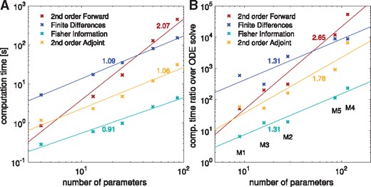
Scaling of computation times of the four investigated methods to compute or approximate the Hessian, (at global optimum for each model) including linear fits and their slopes. All reported computation times were averaged over 10 runs. (A) Model M5 was taken and the number of parameters was fixed to different values. (B) The ratio of the computation times for Hessians or their approximations over the computation time for solving the original ODE is given for the five models from Table 1

We also evaluated whether the same scaling holds across models (Fig. 1B). Interestingly, we found similar but slightly higher slopes for all considered methods, although the number of state variables between models differs substantially. This suggests that in practice the number of parameters is indeed a dominating factor. Overall, second order adjoint sensitivity analysis was the most efficient method for the evaluation of the Hessian.

3.4 Accuracy

To assess the accuracy of Hessians and their approximations provided by the different methods, we compared the results at the global optimum. In general, we observed a good agreement of Hessians computed using second order adjoint and forward sensitivity analysis (Fig. 2A). For the Hessian computed by finite difference, we found—as expected—numerical errors (Fig. 2B), which depended non-trivially on the combination of ODE solver accuracy and the step size of the finite differences. The FIM usually differed substantially from the Hessians, even though this approximation is often considered to be good close to a local optimum (Fig. 2C).

Fig. 2.

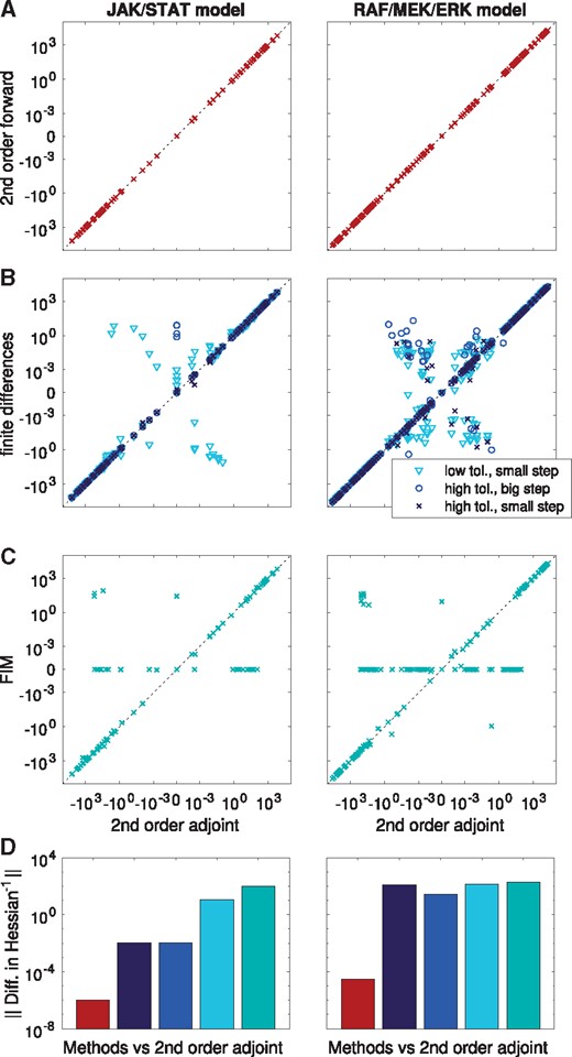
Accuracy of different methods to compute or approximate the Hessian at the global optimum for the models M2 and M3. Each point represents the numerical value of one Hessian entry as computed by two different methods: (A) Second order forward analysis versus second order adjoint analysis. (B) Finite differences (different finite difference step sizes and ODE solver tolerances were considered) versus second order adjoint analysis. (C) FIM versus second order adjoint analysis. All computations were carried out with relative and absolute tolerances set to 10^–11 and 10^–14, respectively. For finite differences, lower accuracies of 10^–7 and 10^–10 were tested, together with the step sizes 10^–5 and 10^–2. (D) Operator norm of the differences in the inverse of the regularized Hessians computed with second order adjoint sensitivity analysis compared to five considered methods (second forward sensitivity analysis, finite differences with different tolerances and step sizes, FIM)

Since most optimization algorithms internally compute a Newton-type update $\Delta \theta =-H^{-1}g$⁠, in which H is the Hessian and g is the gradient, we also evaluated the quality of the Hessian pre-image. For this purpose, we compared the inverses of the regularized Hessians computed with different methods with the one computed using second order adjoint sensitivity analysis in the operator norm. If the Hessian was not invertible, we used the Moore-Penrose-Pseudoinverse. This analysis revealed that the pre-images from second order forward and adjoint sensitivity analysis coincide well, whereas those from finite differences and the FIM differed substantially from the results based on second order sensitivity analysis (Fig. 2D).

In combination, our assessment of scaling and accuracy revealed that second order adjoint sensitivity analysis provides the most scalable approach to obtain accurate Hessians. Rough approximations of the Hessian in terms of the FIM could however be computed at a lower computational cost.

3.5 Optimization

As our results revealed a trade-off between accuracy and computation time for computating Hessians, we investigated how this affects different optimization algorithms. To this end we compared Newton and quasi-Newton variants of the IP algorithm and the TR-reflective algorithm:

• Residuals and their sensitivities were computed with first order forward sensitivity analysis and provided to the least-squares algorithm lsqnonlin, which used the TR-reflective algorithm.

• Gradient and FIM were computed using first order forward sensitivity analysis and provided to fmincon, which used the TR-reflective algorithm.

• Gradient and Hessian were computed with second order adjoint sensitivity analysis. A positive definite transformation of the Hessian was provided to fmincon, using the TR-reflective algorithm (which needs a positive definite Hessian to work).

• Gradients were calculated using first order forward sensitivity analysis and provided to fmincon, using the IP algorithm with a BFGS approximation of the Hessian.

• Gradient and FIM were computed with first order forward sensitivity analysis and provided to fmincon, using the IP algorithm.

• Gradients and Hessians were calculated with second order adjoint sensitivity analysis and provided to fmincon, using the IP algorithm.

The optimization study was carried out using the MATLAB toolbox PESTO for the models M2 and M3. For each of these local optimization methods, we performed four multi-start local optimizations with different initializations and 200 starting points each. A detailed list of the settings of the local optimization methods can be found in the Supplementary Section S2.

We considered the least-squares algorithm lsqnonlin as gold standard for the considered problem class, as this method has previously been shown to be very efficient (Raue et al., 2013b). Here, we studied the effect of using exact Hessians on the optimization algorithms TR-reflective and IP implemented in fmincon. As performance measure of the optimization methods, we considered the computation time per converged start (i.e. starts which reached the global optimum), the total number of converged starts and the number of optimization steps.

The least-square solver lsqnonlin outperformed, as expected, the constraint optimization method fmincon (Fig. 3 and Supplementary Fig. S1). Among the constraint optimization methods, the methods using exact Hessians computed using the second order adjoint method, performed equal or better than the alternatives regarding overall computational efficiency (Fig. 3A). Indeed, the methods reached a higher percentage of converged starts (Fig. 3B and Supplementary Fig. S1) than fmincon using the FIM or the BFGS scheme. This is important, as convergence of the local optimizer is often the critical property (Raue et al., 2013b). In addition, the number of necessary function evaluations was reduced (Fig. 3C). Furthermore, we found differences in convergence and computational efficiency for fmincon, depending on the chosen algorithm.

Fig. 3.

Performance measures of different local optimization methods [lsqnonlin with TR algorithm and fmincon with TR and IP algorithm, using either Hessians (H), FIM, or the BFGS scheme]. The multi-start optimization was carried out multiple times using different starting points for the local optimizations. Mean and standard deviation for (A) the ratio of computation time over converged optimization starts and (B) the number of converged starts are shown. (C) Median and standard deviation of the number of optimization steps over all optimization runs

3.6 Profile likelihood calculation

To assess the benefits of Hessians in uncertainty analysis, we compared the performance of optimization- and integration-based profile calculation methods for the models M2 and M3. For the optimization-based approach, we employed the algorithm implemented in PESTO, which uses first order proposal with adaptive step-length selection (Boiger et al., 2016). We compared the local optimization strategies described in Section 3.5 (omitting the methods based on the FIM, due to their poor performance). For the hybrid approach, we used MATLAB default tolerances for ODE integration. We compared the hybrid scheme using Hessians and the FIM. All profiles were computed to a confidence level of 95%.

The comparison of the profile likelihoods calculated using different approaches revealed substantial differences (Fig. 4B and C). The optimization-based approaches worked fine for the JAK/STAT model but mostly failed for the RAF/MEK/ERK model (Fig. 4A). For the RAF/MEK/ERK model, only fmincon with the TR-reflective algorithm and exact Hessians worked reliably among the optimization-based methods. Even lsqnonlin yielded inaccurate results for 11 out of 28 parameter profiles. A potential reason is that the tolerances––which were previously also used for optimization––were not sufficiently tight. Purely integration-based methods failed due to numerical problems, e.g. jumps in the profile paths. Even extensive manual tuning and the use of different established ODE solvers (including ode113, ode45, ode23 and ode15s) did not result in reasonable approximations for all profiles. In contrast, the hybrid approach provided accurate profiles for all parameters and all models, when provided with exact Hessians. However, when provided with the FIM, the hybrid approach failed, when it had to perform optimization.

Fig. 4.

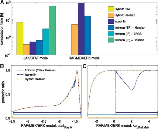
Profile likelihood computation using either the optimization-based method (lsqnonlin or fmincon with TR or IP algorithm and Hessian or BFGS approximation), or the hybrid method with either FIM or Hessian. (A) Total computation time for all profiles of the considered models. Three methods failed to compute profiles for the RAF/MEK/ERK model. Thus, their computation times are not depicted. (B) A profile of the RAF/MEK/ERK model, the three remaining methods in good agreement with each other, with confidence intervals to a confidence level of 95% depicted below. (C) A profile of the RAF/MEK/ERK model, for which lsqnonlin failed to compute the profile, with confidence intervals to a confidence level of 95% depicted below

In addition to the accuracy, also the computation time of the methods differed substantially. The hybrid method using exact Hessians was substantially faster than the remaining methods (Fig. 4A and Supplementary Fig. S6). The second fastest method was the optimization-based approach using the Hessian and the TR-reflective algorithm for optimization. lsqnonlin was slightly slower and fmincon using the IP algorithm substantially slower (for both, the BFGS scheme and Hessian), although they––as mentioned above––did not provide accurate profiles.

Overall, the proposed hybrid approach using exact Hessians outperformed all other methods. Compared to the best reliable competitor (optimization-based profile calculation using fmincon with the TR-reflective algorithm and exact Hessians), the computation time was reduced by more than a factor of two. This is substantial for such highly optimized routines and outlines the potential of exact Hessians for uncertainty analysis.

4 Discussion

Mechanistic ODE models in systems and computational biology rely on parameter values, which are inferred from experimental data. In this manuscript, we showed that the efficiency of some of the most common methods in parameter estimation can be improved by providing exact second order derivatives. We presented second order adjoint sensitivity analysis, a method to compute accurate Hessians at low computational cost, i.e. the method scales linearly in the number of model parameters and state variables. We also provide a ready-to-use implementation thereof in the freely available toolbox AMICI.

We showed that second order adjoint sensitivity analysis possesses better scaling properties than common methods to compute Hessians while yielding accurate results, rendering it a promising alternative to existing techniques. Moreover, we demonstrated that state-of-the-art constraint optimization algorithms yield more robust results when using exact Hessians. For the computation of profile likelihoods, we demonstrated that Hessians can improve computation time and robustness of various state-of-the-art methods. Furthermore, we presented a hybrid method for profile computation, which can efficiently handle problems that are poorly locally identifiable and have ill-conditioned Hessians. We also provided an implementation of this method in the freely available PESTO. Although being a reliable approach for uncertainty analysis (Fröhlich et al., 2014), profile likelihoods are often disregarded due to their high computational effort. The presented hybrid method based on exact Hessians is an approach the tackle this problem, as already the rudimentary implementation used in this study outperformed all established approaches.

The analysis of the optimizer performance revealed that least-squares algorithms (such as lsqnonlin), which exploit the problem structure, are difficult to outperform. Many parameter estimation problems considered in systems biology do however not possess this structure. This is for instance the case for problems with additional constraints, applications considering the chemical master equation (Fröhlich et al., 2016), or ODE-constrained mixture models (Hasenauer et al., 2014). For these problem classes, the constraint TR and IP optimization algorithms as implemented in fmincon are the state-of-the-art methods. Additionally, new algorithms, which can exploit the additional curvature information, available through exact Hessian computation, in novel ways are steadily developed (Fröhlich et al., 2017b). Either directions of negative curvature can be used to escape saddle-points efficiently (Dauphin et al., 2014), or third-order approximations of the objective functions are constructed iteratively from the Hessians along the trajectory of optimization to improve the convergence order (Martinez and Raydan, 2017). Another approach would be using a quasi-Newton-method in the beginning of the optimization process and switching to exact Hessians as soon as the algorithm comes close to a first-order stationary point. This might improve the computational performance, since curvature information is typically more helpful in vicinity of a local optimum. Some of these approaches might outperform current optimization strategies, which are not designed to exploit e.g. directions of negative curvature that may be present in non-convex problems. These methods will be particularly interesting subjects of further studies when being combined with second order adjoint sensitivity analysis.

Besides optimization and profile likelihood calculation, Hessians can also be used for local approximations of the likelihood function, which facilitates the efficient assessment of practical identifiability properties and the approximation of the parameter confidence intervals. In addition, the Hessian can be employed by sampling methods, which consider uncertainties from a more Bayesian point of view. Also bootstrapping methods profit from Hessians, as optimization is improved. Hence, the approaches presented here may accelerate various uncertainty analysis methods and make their application feasible for model sizes, for which these methods have not been applicable before.

While this study focused on the efficient calculation of the Hessian, second order adjoint sensitivity analysis can also be used to compute Hessian vector products. This information can be exploited by optimization methods such as truncated Newton (Nash, 1984) or accelerated conjugate gradient (Andrei, 2009) algorithms, which are suited for large-scale optimization problems. These are a few examples to illustrate how the presented results may pave the way for future improvements.

Funding

This work was supported by the German Research Foundation (DFG) through the Graduate School of Quantitative Biosciences Munich (QBM; F.F.) and through the European Union’s Horizon 2020 research and innovation program under grant agreement no. 686282 (J.H. and P.S.).

Conflict of Interest: none declared.