MicroPheno: predicting environments and host phenotypes from 16S rRNA gene sequencing using a k-mer based representation of shallow sub-samples

Abstract

Motivation

Microbial communities play important roles in the function and maintenance of various biosystems, ranging from the human body to the environment. A major challenge in microbiome research is the classification of microbial communities of different environments or host phenotypes. The most common and cost-effective approach for such studies to date is 16S rRNA gene sequencing. Recent falls in sequencing costs have increased the demand for simple, efficient and accurate methods for rapid detection or diagnosis with proved applications in medicine, agriculture and forensic science. We describe a reference- and alignment-free approach for predicting environments and host phenotypes from 16S rRNA gene sequencing based on k-mer representations that benefits from a bootstrapping framework for investigating the sufficiency of shallow sub-samples. Deep learning methods as well as classical approaches were explored for predicting environments and host phenotypes.

Results

A k-mer distribution of shallow sub-samples outperformed Operational Taxonomic Unit (OTU) features in the tasks of body-site identification and Crohn’s disease prediction. Aside from being more accurate, using k-mer features in shallow sub-samples allows (i) skipping computationally costly sequence alignments required in OTU-picking and (ii) provided a proof of concept for the sufficiency of shallow and short-length 16S rRNA sequencing for phenotype prediction. In addition, k-mer features predicted representative 16S rRNA gene sequences of 18 ecological environments, and 5 organismal environments with high macro-F1 scores of 0.88 and 0.87. For large datasets, deep learning outperformed classical methods such as Random Forest and Support Vector Machine.

Availability and implementation

The software and datasets are available at https://llp.berkeley.edu/micropheno.

Supplementary information

Supplementary data are available at Bioinformatics online.

1 Introduction

Microbial communities have important functions relevant to supporting, regulating, and in some cases causing unwanted conditions (e.g. diseases) in their hosts/environments, ranging from organismal environments, such as the human body, to ecological environments, such as soil and water. These communities typically consist of a variety of microorganisms, including eukaryotes, archaea, bacteria and viruses. Due to differences in nutrient availability and environmental conditions, microbial communities from different environments have widely varying taxonomic structures and compositions (Ann Moran, 2015; Armbrust et al., 2015; Fierer, 2017; Pinto et al., 2012).

The human microbiota refers to all microorganisms living in close association with the human body. It is now widely believed that changes in our microbiota correlate with numerous diseases, raising the possibility that manipulation of these communities may be used to treat diseases. The microbiota (particularly the intestinal microbiota) is known to play important roles in healthy humans, including: (i) prevention of pathogen growth, (ii) education and regulation of the host immune system and (iii) providing energy substrates to the host (Lynch and Pedersen, 2016). Consequently, dysbiosis of the human microbiota can promote diseases, including asthma (Arrieta et al., 2015; Marsland et al., 2013), irritable bowel syndrome (Cho and Blaser, 2012; Saulnieret al., 2011), Clostridium difficile infection (Cammarota et al., 2014), chronic periodontitis (Jorth et al., 2014; Luo Deng et al., 2017), cutaneous leishmaniasis (Gimblet et al., 2017), obesity (Ridaura et al., 2013; Turnbaugh et al., 2008), chronic kidney disease (Ramezani and Raj, 2014), Ulcerative colitis (Michail et al., 2012) and Crohn’s disease (Gevers et al., 2014; Pascal et al., 2017). The human microbiota appears to play a particularly important role in the development of Crohn’s disease. Crohn’s disease is an inflammatory bowel disease (IBD) with a prevalence of approximately 40 per 100 000 and 200 per 100 000 in children and adults, respectively (Kappelman et al., 2007). Environmental microbial communities also serve important functions, such as nutrient cycling (Gilbert and Neufeld, 2014). For instance, the microbiota living in the ocean account for half of the primary production on the Earth (Ann Moran, 2015). The soil microbiome surrounding the root of plants impacts plant fertility and growth (Chaparro et al., 2012).

The starting point of many microbiome studies is commonly 16S rRNA gene sequencing of microbial samples (Hamady and Knight, 2009). The 16S rRNA gene is highly conserved across bacteria and archaea, includes both conserved regions, against which universal species-independent polymerase chain reaction primers can be directed, and nine hypervariable regions (V1–V9), which allow differential identification of taxon identities and relative abundances (Michael Janda et al., 2007). After sequencing, the obtained data are usually processed with bioinformatics software such as Quantitative Insights Into Microbial Ecology (QIIME) (Gregory Caporaso et al., 2010; Lawley and Tannock, 2017), Mothur (Schloss et al., 2009) or Usearch (Edgar et al., 2011) and clustered into groups of closely related sequences, referred to as operational taxonomic units (OTUs). Later in Section 1.2, we discuss the pros and cons of OTU features in detail. The low cost of 16S rRNA gene sequencing is one of the primary reasons for its widespread use in microbiome research. However, 16S rRNA sequencing has several disadvantages compared to shotgun metagenome sequencing, detailed in the Supplemental Material, such as its inability to resolve functions, and accordingly functional variations within individual taxa (Pollock et al., 2018).

1.1 Machine learning for environments or host phenotypes classification

Several recent studies predicted the environment or host phenotypes using 16S gene sequencing data for body-sites (Knights et al., 2011; Statnikov et al., 2013), disease state (Duvallet et al., 2017; Eck et al., 2017; Xu et al., 2016), ecological environment quality status prediction (Cordier et al., 2017) and subject prediction for forensic science (Fierer et al., 2010; Schmedes et al., 2018). In all, OTUs served as the main input feature for the downstream machine learning algorithms. Random Forest (RF) and then, ranking second, linear Support Vector Machine (SVM) classifiers were reported as the most effective classification approaches in these studies (Carrieri et al., 2017; Duvallet et al., 2017; Pasolli et al., 2016; Statnikov et al., 2013).

Related prior work on body-site classification (Knights et al., 2011; Statnikov et al., 2013) used the following datasets: Costello Body Habitat (CBH—6 classes), Costello Skin Sites (CSS—12 classes) (Costello et al., 2009), and Pei Body Site (PBS—4 classes) (Statnikov et al., 2013). An extensive comparison of classifiers for body-site classification over CBH, CSS and PBS on top of OTU features has been performed by Statnikov et al. (2013). The best accuracy levels measured by relative classifier information (RCI) achieved by using OTU features are reported as 0.784, 0.681 and 0.647 for CBH, CSS and RCI, respectively. Due to the insufficiency of the number of samples (on average 57 samples per class for CBH, CSS and PBS) as well as the unavailability of raw sequences for some of the datasets mentioned above, instead of using the same dataset we replicate the state-of-the-art approach suggested in Statnikov et al. (2013), i.e. RF and SVM over OTU features for a larger dataset [Human Microbiome Project (HMP) dataset]. We then compare OTU features with k-mer representations. Working on a larger dataset allows for a more meaningful investigation and better training for deep learning approaches.

Detecting disease status based on 16S gene sequencing is becoming more and more popular, with applications in the prediction of Psoriasis (151 samples for 3 classes—best accuracy: 0.225), IBD (patients: 49 samples, healthy: 59—best AUC: 0.95) (Xu et al., 2016) and (patients: 91 samples, healthy: 58 samples—best AUC: 0.92) (Eck et al., 2017). Similar to body-site classification datasets, the datasets used for disease prediction were also relatively small. In this article, we use the Crohn’s disease dataset (Gevers et al., 2014) with 1359 samples (patients: 731 samples, negative class: 628 samples) for evaluating our proposed method and then compare it with the use of OTU features.

We focus on machine learning approaches for classification of environments or host phenotypes of 16S rRNA gene sequencing data, which is the most popular and cost-effective sequencing method for the characterization of microbiome to date (Pasolli et al., 2016; Pollock et al., 2018). Studies on the use of machine learning for predicting microbial phenotype instead of environments/host phenotype (Dutilh et al., 2013; Ross et al., 2013), as well as predictions based on shotgun metagenome and whole-genome microbial sequencing are beyond the scope of this article, although we believe that one may easily adapt the proposed approach to shotgun metagenomics, similar to the study by Cui et al. on IBD prediction (Cui and Zhang, 2013).

Recently, deep learning methods became popular in various applications of machine learning in bioinformatics (Asgari and Mofrad, 2015; Min et al., 2016) and in particular in microbiome research (Ditzler et al., 2015). However, to the best of our knowledge, this is the first study exploring environment and host phenotype prediction from 16S rRNA gene sequencing data with deep learning approaches.

1.2 16S rRNA gene sequence representations

OTU representation

As reviewed in Section 1.1, prior machine learning works on environment/host phenotype prediction have been mainly using OTU representations as the input features to the learning algorithm. Although there exist non-OTU based pipelines for 16S rRNA sequence analysis [e.g. DADA-2 (Callahan et al., 2016)], almost all popular 16S rRNA sequence processing pipelines cluster sequences into OTUs based on their sequence similarities, utilizing a variety of algorithms (Lawley and Tannock, 2017; Nguyen et al., 2016). QIIME allows OTU-picking using three different strategies: (i) closed-reference OTU-picking: sequences are compared against a marker gene database [e.g. Greengenes (McDonald et al., 2012) or SILVA (Quast et al., 2012)] to be clustered into OTUs and then the sequences different from the reference genomes beyond a certain sequence identity threshold are discarded. (ii) Open-reference OTU-picking: the remaining sequences after a closed-reference calling go through a de novo clustering. This allows for using the whole sequences as well as capturing sequences belonging to new communities, which are absent in the reference databases (Rideout et al., 2014). (iii) Pure de novo OTU-picking: sequences (or reads) are only compared among themselves and no reference database is used. The third strategy is more appropriate for novel species absent in the current reference. Although OTU clustering reduces the analysis of millions of reads to working with only thousands of OTUs and simplifies the subsequent phylogeny estimation and multiple sequence alignment, OTU representations have several shortcomings: (i) all three OTU-picking strategies involve massive amounts of sequence alignments either to the reference genomes (in closed-/opened-reference strategies) or to the sequences present in the sample (in open-reference and de novo strategies) which makes them very expensive (Cai et al., 2017) in comparison with reference-free/alignment-free representations. (ii) Overall sequence similarity is not a proper condition for grouping sequences and OTUs can be phylogenetically incoherent. For instance, a single mutation between two sequences is mostly ignored by OTU-picking algorithms. However, if the mutation does not occur within the sample, it might be a signal for assigning a new group. In addition, several mutations within a group most likely are not going to be tolerated by OTU-picking algorithms. However, having the same ratio across samples may suggest that the mutated sequences belong to the same group (Koeppel and Wu, 2013; Nguyen et al., 2016). (iii) The number of OTUs and even their contents are very sensitive to the pipeline and parameters, and this makes them difficult to reproduce (He et al., 2015).

1.2 k-mer representations

k-mer count vectors have been shown to be suitable input features for performing machine learning on biological sequences for a variety of bioinformatics tasks (Marçais and Kingsford, 2011). In particular, k-mer count features have been used for taxonomic classifications of microbial 16S and metagenome datasets (Kawulok and Deorowicz, 2015; McHardy et al., 2007; Menzel and Krogh, 2015; Patil et al., 2011; Vervier et al., 2016; Wood and Salzberg, 2014). However, to the best of our knowledge, k-mer features have not been explored for phenotypical and environmental characterizations of 16S rRNA sequence data.

In this article, we propose using k-mer representations of shallow sub-samples for predicting environments and host phenotypes from 16S rRNA sequences. Our approach is fast, reference-free and alignment-free, while contributing to building accurate classifiers outperforming conventional OTU features in body-site identification and Crohn’s disease classification. We propose a bootstrapping framework to investigate the sufficiency of shallow sub-samples for the prediction of the phenotype of interest, which proves the sufficiency of short-length and shallow sequencing of 16S rRNA. In addition, we explore deep learning methods as well as classical approaches for classification. Furthermore, we demonstrate the value of Principal Component Analysis (PCA), t-Distributed Stochastic Neighbor Embedding (t-SNE) and supervised deep representation learning for visualization of microbial samples/sequences of different phenotypes. We also show that k-mer features can be used to predict representative 16S rRNA gene sequences from 18 ecological environments and 5 organismal environments with high macro-F1s.

2 Materials and methods

2.1 Datasets

Body-site identification

We employ the 16S rRNA gene sequence dataset provided by the NIH HMP (Huttenhower et al., 2012; Jane et al., 2009) (Available at http://hmpdacc.org/HM16STR/). In particular, we use processed, annotated 16S rRNA gene sequences of up to 300 healthy individuals, each sampled at four major body-sites (oral, airways, gut and vagina) and up to three time points. For each major body-site, a number of sub-sites were sampled. We focus on five body sub-sites: anterior nares (nasal) with 295 samples, saliva (oral) with 299 samples, stool (gut) with 325 samples, posterior fornix (urogenital) with 136 samples and mid-vagina (urogenital) with 137 samples, in total 1192 samples. These body-sites are selected to represent differing levels of spatial and biological proximity to one another, based on relevance to pertinent human health conditions potentially influenced by the human microbiome. To compare k-mer based approach with state-of-the-art OTU features, we collect the closed-reference OTU representations of the same samples in HMP (Huttenhower et al., 2012) (Available at https://qiita.ucsd.edu/study/descriptipn/1928) obtained using the QIIME pipeline (Rideout et al., 2014).

Crohn’s disease prediction

For the classification of Crohn’s disease, we use the 16S rRNA dataset described in (Gevers et al., 2014) (Available at: https://www.ncbi.nlm.nih.gov/bioproject/PRJEB13679), which is currently the largest pediatric Crohn’s disease dataset available. This dataset includes annotated 16S rRNA gene sequence data for 731 pediatric (≤17 years old) patients with Crohn’s disease and 628 samples verified as healthy or diagnosed with other diseases, making a total of 1359 samples. Sequencing here was targeted towards the V4 hypervariable region of the 16S rRNA gene. Similar to the body-site dataset, to compare the k-mer based approach with the approach based on OTU features, we collect the OTU representations of the same samples from Qiita repository (Available at https://qiita.ucsd.edu/study/description/1939) obtained using QIIME pipeline (Rideout et al., 2014).

Predicting the environment for representative 16S rRNA gene sequences

MetaMetaDB provides a comprehensive dataset of representative 16S rRNA sequences of various ecological and organismal environments, collected from existing 16S rRNA databases spanning almost 181 million raw sequences. In the MetaMetaDB pipeline, low-quality nucleotides, adapters, ambiguous sequences, homopolymers, duplicates and reads shorter than 200 bp, as well as chimeras have been removed and 16S rRNA sequences were clustered with 97% identity, generating 1 241 213 representative 16S rRNA sequences marked by their environment (Chia Yang and Iwasaki, 2014). MetaMetaDB divides its ecological environments into 34 categories and its organismal environments into 28 categories. We create three datasets, which are subsets of MetaMetaDB, to investigate the discriminative power of k-mers in predicting microbial habitats. Since the sequences in MetaMetaDB were already filtered and semi-identical sequences removed, OTU-picking would not be required, as it would result in an almost one-to-one mapping between the sequences and OTUs (we verified this using QIIME).

Ecological environment prediction: MetaMetaDB is imbalanced in terms of the number of representative sequences per environment. For this study, we pick the ecological environments with more than 10 000 samples, ending up with corresponding to 18 classes of ecological environments: activated sludge, ant fungus garden, aquatic, bioreactor, bioreactor sludge, compost, food, food fermentation, freshwater, freshwater sediment, groundwater, hot springs, hydrocarbon, marine, marine sediment, rhizosphere, sediment and soil (Datasets and descriptions are available at http://mmdb.aori.u-tokyo.ac.jp/download.html). We make two datasets out of the sequences in these environments by stratified sampling: ECO-18K containing 1000 randomly selected instances per class (a total of 18 K sequences) and ECO-180K, which is 10 times larger than ECO-18K, i.e. contains 10 000 randomly selected instances per class (a total of 180 K sequences).

Organismal environment prediction: From the organismal environments in MetaMetaDB, we select a subset containing gut microbiomes of five different organisms (bovine gut, chicken gut, human gut, mouse gut and termite gut) and down-sampled each class to the size of the smallest class by stratified sampling, resulting in 620 samples per class and a total of 3100 sequences. We call this dataset 5GUTS-3100.

2.2 MicroPheno computational workflow

We describe using deep learning and classical methods for classification of the environments or host phenotypes of microbial communities using k-mer frequency representations obtained from shallow sub-sampling of 16S rRNA gene sequences. We propose a bootstrapping framework to confirm the sufficiency of using a small portion of the sequences within a 16S rRNA sample for determining the underlying phenotype. The MicroPheno computational workflow has the following steps (Fig. 1): (i) to find the proper size N for the sample, such that it stays representative of the data and produces a stable k-mer profile, the 16S rRNA sequences go through a bootstrapping phase. (ii) Afterwards, the sub-sampled sequences are used to find the best value for k for classification, to produce the k-mer representations of the samples. (iii) The k-mer representations are used for classification with deep neural networks (DNN), RF and linear SVM. (iv) Finally, the k-mer representations as well as the supervised representations trained using DNNs are used for visualization of the 16S rRNA gene sequences or samples. In what follows, these steps are explained in detail.

Fig. 1.

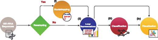
The components and the data flow in the MicroPheno computational workflow

Bootstrapping: Confirming the sufficiency of only a small portion of 16S rRNA sequences for environment or host phenotype classification is important because (i) sub-sampling reduces the preprocessing run-time, and (ii) more importantly, it proves that even a shallow 16S rRNA sequencing is enough. We propose a resampling framework to give us quantitative measures for finding the proper sampling size. Let ${\theta }_k\left(X_i\right)$ be the normalized k-mer distribution of X_i, a set of sequences in the ith 16S rRNA sample. We investigate whether only a portion of X_i, which we represent as ${\tilde{x}}_{ij}$⁠, i.e. jth resample of X_i with sample size N, would be sufficient for producing a proper representation of X_i. To quantitatively find a sufficient sample size for X_i, we propose the following criteria in a resampling scheme. (i) Self-consistency: resamples for a given size N from X_i produce consistent ${\theta }_k\left({\tilde{x}}_{ij}\right)$’s, i.e. resamples should have similar representations. (ii) Representativeness: resamples for a given size N from X_i produce ${\theta }_k\left({\tilde{x}}_{ij}\right)$’s similar to ${\theta }_k\left(X_i\right)$⁠, i.e. similar to the case where all sequences are used.

We quantitatively define self-inconsistency and unrepresentativeness and seek parameter values that minimize them. We measure the self-inconsistency ($\overline{D_S}$) of the resamples’ representations by calculating the average Kullback–Leibler divergence among normalized k-mer distributions for N_R resamples (here $N_R=1\mathrm{0}$⁠) with sequences of size N from the ith 16S rRNA sample:

$${\overline{D_S}}_i(N,k,N_R)=\frac{1}{N_R(N_R-1)}\sum _{\stackrel{\forall p,q}{(p\ne q)}\in \{1,2,\dots ,N_R\}}{D}_{KL}\left({\theta }_k\right({\tilde{x}}_{ip}),{\theta }_k({\tilde{x}}_{iq}\left)\right),$$

where $\left|\widetilde{x_{il}}\right|=N$⁠; $\forall l\in \{1,2,\dots ,N_R\}$⁠. We calculate the average of the values of ${\overline{D_S}}_i(N,k,N_R)$ over the M different 16S rRNA samples:

$$\overline{D_S}(N,k,N_R)=\frac{1}{M}\sum _{i=1}^M{\overline{D_S}}_i(N,k,N_R).$$

We measure the unrepresentativeness (⁠$\overline{D_R}$⁠) of the resamples by calculating the average Kullback–Leibler divergence between normalized k-mer distributions for N_R resamples (N_R=10) with size N and using all the sequences in X_i for the ith 16S rRNA sample:

$${\overline{D_R}}_i(N,k,N_R)=\frac{1}{N_R}\sum _{\forall p\in \{1,2,\dots ,N_R\}}{D}_{KL}\left({\theta }_k\right({\tilde{x}}_{ip}),{\theta }_k(X_i\left)\right),$$

where $\left|\widetilde{x_{il}}\right|=N$⁠; $\forall l\in \{1,2,\dots ,N_R\}$⁠. We calculate the average over ${\overline{D_R}}_i(N,k)$’s for the M 16S rRNA samples:

$$\overline{D_R}(N,k,N_R)=\frac{1}{M}\sum _{i=1}^M{\overline{D_R}}_i(N,k,N_R).$$

For the experiments on body-site and the dataset for Crohn’s disease, we measure self-inconsistency $\overline{D_S}$ and unrepresentativeness $\overline{D_R}$ for N_R = 10 and M = 10 for any $8\ge k\ge 3$ with sampling sizes ranging from 20 to 10 000. Each point in Figure 4 represents the average of 100 (⁠$M\times N_R$⁠) resamples belonging to M randomly selected 16S rRNA samples, each of which is resampled N_R = 10 times. Since in the ecological and organismal datasets each sample is a single sequence, the bootstrapping step is skipped.k-mer representation: We propose using the l1 normalized k-mer distribution of 16S rRNA sequences as input features for machine learning classification algorithms as well as visualization. Normalizing the representation allows for having a consistent representation, even when the sampling size is changed. For each k-value, we pick a sampling size that gives us a self-consistent and representative representation measured by $\overline{D_S}(N,k,N_R)$ and $\overline{D_R}(N,k,N_R)$⁠, respectively, as explained above.

Classification: RFs and linear SVM are the state-of-the-art classical approaches for categorical prediction on 16S rRNA sequences (Duvallet et al., 2017; Pasolli et al., 2016; Statnikov et al., 2013) and in general for many machine learning problems in bioinformatics (Olson et al., 2017). These two approaches, which are respectively instances of non-linear and linear classifiers, are both adopted in this study. In addition to these classical approaches, we also evaluate the performance of DNN classifiers in predicting environments and host phenotypes.

We evaluate and tune the model parameter in a stratified 10-fold cross-validation scheme. To ensure optimizing for both precision and recall, we optimize the classifiers for the harmonic mean of precision and recall, i.e. F1. In particular, to give equal importance to the classification categories, specifically when we have imbalanced classes, we use macro-F1, which is the average of F1’s over categories. Finally the evaluation metrics are averaged over the folds and the standard deviation is also reported. We provide both micro and macro-metrics which are averaged over instances and over categories, respectively.

Classical learning algorithms: We use a one-versus-rest strategy for multi-class linear SVM (Suykens and Vandewalle, 1999) and tune parameter C, the penalty term for regularization. RF (Breiman, 2001) classifiers are tuned for (i) the number of decision trees in the ensemble, (ii) the number of features for computing the best node split and (iii) the function to measure the quality of a split.

Deep learning: We use the Multi-Layer-Perceptrons (MLP) neural network architecture with several hidden layers using Rectified Linear Unit (ReLU) as the nonlinear activation function. We use the softmax activation function at the last layer to produce the probability vector that can be regarded as representing posterior probabilities (Goodfellow et al., 2016). To avoid overfitting, we perform early stopping and also use dropout at hidden layers (Srivastava et al., 2014). A schematic visualization of our neural networks is depicted in Figure 2. Our objective is minimizing the loss, i.e. cross entropy between output and the one-hot vector representation of the target class. The error (the distance between the output and the target) is used to update the network parameters via a back-propagation algorithm using Adaptive Moment Estimation (Adam) as the optimizer (Kingma and Lei Ba, 2015). We start with a single hidden layer and incrementally increase the number of layers with systematic exploration of the number of hidden units and dropout rates to find a proper architecture. We stop adding layers when increasing the number of layers does not result in achieving a higher macro-F1 anymore. In addition, for the visualization of samples we use the output of the $(n-1)\text{th}$ hidden layer. Later in the results DNN-nL is a short form for a MLP neural network with n layers.

Fig. 2.

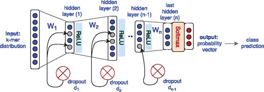
General architecture of the MLP neural networks that have been used in this study for multi-class classification of environment and host phenotypes

Visualization: To project 16S rRNA sequencing samples to 2D for visualization purposes, we explore PCA (Jolliffe, 1986) as well as t-SNE (Van Der Maaten and Hinton, 2008), as instances of respectively linear and non-linear dimensionality reduction methods. In addition, we explore the use of supervised deep representation learning in visualization of data (Bengio et al., 2013), i.e. we visualize the activation function of the last hidden layer of the neural network trained for prediction of environments or host phenotypes to be compared with unsupervised methods. The visualizations help in obtaining a better understanding on how samples are distributed in a high dimensional space and how neural networks can obtain a transformation that separates different categories. More details on visualization methods are provided as Supplementary Materials.

Implementations  : MicroPheno uses implementations of RF, SVM, t-SNE and PCA in the Python library scikit-learn (Pedregosa and Varoquaux, 2011), and DNNs are implemented in the Keras (https://keras.io/) deep learning framework using the TensorFlow back-end.

3 Results

In this section, the results are organized based on datasets. As discussed in Section 2.2, we have several choices in each step in the computational workflow: choosing the value of k in k-mer, the sampling rate and the classifiers. To explore the parameter space more systematically, we followed the steps demonstrated in Figure 3. (i) In the first step, for each value of $8\ge k\ge 3$⁠, we pick a stable sample size based on the output of bootstrapping. (ii) We perform the classification task using tuned RF for different k-values and their selected sampling sizes based on bootstrapping. We selected RF, because we found it easy to tune and because it oftentimes outperforms linear SVM (Olson et al., 2017; Statnikov et al., 2013). (iii) As the third step, for a selected k, we investigate the role of sampling size (N) in classification. (iv) Finally, we compare different classifiers for the selected k and N. We also compare the performance of our proposed k-mer features with that of OTU features in classification tasks.

Fig. 3.

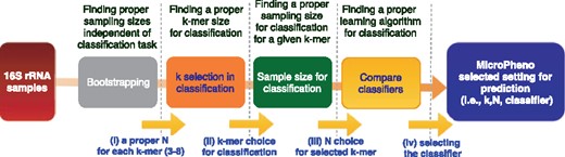
Steps we take to explore parameters for the representations, and how we choose the classifier for prediction of the phenotype of interest in this study

3.1 Body-site identification and Crohn’s disease prediction

(i) Bootstrapping for sampling rate selection for k-mers: Higher k-values require higher sampling rates to produce self-consistent and representative representations (Fig. 4 for body-site dataset). As the structure of the curve for Crohn’s disease dataset is similar to the body-site dataset, to avoid redundancy, the figure for Crohn’s disease is provided as Supplementary Material. For each k, we consider a certain threshold on $\overline{D_S}$ and $\overline{D_R}$⁠, to ensure selecting a sampling size resulting in self-consistent and representative representations.

Fig. 4.

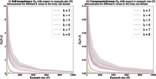
Measuring (i) self-inconsistency (⁠$\overline{D_S}$⁠) and (ii) unrepresentativeness (⁠$\overline{D_R}$⁠) for the body-site dataset. Each point represents an average of 100 resamples belonging to 10 randomly selected 16S rRNA samples. Higher k-values require higher sampling rates to produce self-consistent and representative samples

(ii) Classification for different values of k with a sampling size selected based on the output of bootstrapping: Interestingly, using only 3-mer features with a very low sampling rate (⁠$\approx$20/15 000 = 0.0013) provides a relatively high performance for 5-way body-site classification (Table 1). The value of macro-F1 increases with the value of k from 3 to 6, but increasing k further than that does not have any additional effect on macro-F1 (Table 1, body-site dataset, step (ii)). For Crohn’s disease Choosing k = 6 with a sampling size of 2000 (≈2000/38 000 = 0.05) provided a macro-F1 of 0.75 which is the minimum k with top performance (Table 1, Crohn’s disease dataset, step (ii)).

Table 1.

The results for classification of major body-sites as well as Crohn’s disease prediction using k-mer representations

Dataset	Step	Representation	Resample size	Classifier	Micro-metrics (averaged over samples)			Macro-metrics (averaged over classes)
					Precision	Recall	F1	Precision	Recall	F1
Body-site (≈15 000 reads/ sample)	(ii)	3-mers	20	RF	0.84 ± 0.02	0.84 ± 0.02	0.84 ± 0.02	0.75 ± 0.03	0.75 ± 0.03	0.74 ± 0.03
		4-mers	100		0.86 ± 0.03	0.86 ± 0.03	0.86 ± 0.03	0.77 ± 0.03	0.77 ± 0.03	0.77 ± 0.03
		5-mers	500		0.89 ± 0.02	0.89 ± 0.02	0.89 ± 0.02	0.82 ± 0.03	0.82 ± 0.03	0.82 ± 0.03
		6-mers	2000		0.91 ± 0.03	0.91 ± 0.03	0.91 ± 0.03	0.85 ± 0.05	0.85 ± 0.04	0.84 ± 0.05
		7-mers	5000		0.91 ± 0.03	0.91 ± 0.03	0.91 ± 0.03	0.85 ± 0.05	0.85 ± 0.05	0.85 ± 0.05
		8-mers	8000		0.9 ± 0.03	0.9 ± 0.03	0.9 ± 0.03	0.85 ± 0.05	0.84 ± 0.05	0.84 ± 0.05
Crohn’s disease (≈38 000 reads/ sample)	(ii)	3-mers	20	RF	0.62 ± 0.05	0.62 ± 0.05	0.62 ± 0.05	0.62 ± 0.05	0.61 ± 0.05	0.61 ± 0.05
		4-mers	100		0.7 ± 0.05	0.7 ± 0.05	0.7 ± 0.05	0.69 ± 0.05	0.69 ± 0.05	0.69 ± 0.05
		5-mers	500		0.74 ± 0.05	0.74 ± 0.05	0.74 ± 0.05	0.74 ± 0.05	0.74 ± 0.05	0.74 ± 0.05
		6-mers	2000		0.75 ± 0.04	0.75 ± 0.04	0.75 ± 0.04	0.75 ± 0.04	0.75 ± 0.04	0.75 ± 0.04
		7-mers	5000		0.75 ± 0.04	0.75 ± 0.04	0.75 ± 0.04	0.75 ± 0.04	0.75 ± 0.04	0.75 ± 0.04
		8-mers	8000		0.75 ± 0.04	0.75 ± 0.04	0.75 ± 0.04	0.75 ± 0.04	0.75 ± 0.04	0.75 ± 0.04
Body-site	(iii)	6-mers	100	RF	0.89 ± 0.02	0.89 ± 0.02	0.89 ± 0.02	0.82 ± 0.04	0.82 ± 0.03	0.81 ± 0.03
			1000		0.9 ± 0.03	0.9 ± 0.03	0.9 ± 0.03	0.83 ± 0.04	0.83 ± 0.04	0.83 ± 0.04
			2000		0.91 ± 0.03	0.91 ± 0.03	0.91 ± 0.03	0.85 ± 0.05	0.85 ± 0.04	0.84 ± 0.05
			5000		0.9 ± 0.03	0.9 ± 0.03	0.9 ± 0.03	0.85 ± 0.04	0.84 ± 0.04	0.84 ± 0.04
			10 000		0.9 ± 0.03	0.9 ± 0.03	0.9 ± 0.03	0.84 ± 0.05	0.84 ± 0.05	0.84 ± 0.05
			All sequences		0.9 ± 0.03	0.9 ± 0.03	0.9 ± 0.03	0.84 ± 0.05	0.84 ± 0.04	0.84 ± 0.05
Crohn’s disease	(iii)	6-mers	100	RF	0.71 ± 0.04	0.71 ± 0.04	0.71 ± 0.04	0.71 ± 0.04	0.7 ± 0.04	0.7 ± 0.04
			1000		0.75 ± 0.04	0.75 ± 0.04	0.75 ± 0.04	0.76 ± 0.04	0.75 ± 0.04	0.75 ± 0.04
			2000		0.75 ± 0.04	0.75 ± 0.04	0.75 ± 0.04	0.75 ± 0.04	0.75 ± 0.04	0.75 ± 0.04
			5000		0.76 ± 0.04	0.76 ± 0.04	0.76 ± 0.04	0.76 ± 0.04	0.75 ± 0.04	0.75 ± 0.04
			10 000		0.76 ± 0.04	0.76 ± 0.04	0.76 ± 0.04	0.76 ± 0.05	0.75 ± 0.04	0.75 ± 0.05
			All sequences		0.76 ± 0.04	0.76 ± 0.04	0.76 ± 0.04	0.76 ± 0.05	0.75 ± 0.04	0.75 ± 0.05
Body-site	(iv)	6-mers	5000	RF	0.9 ± 0.03	0.9 ± 0.03	0.9 ± 0.03	0.85 ± 0.04	0.84 ± 0.04	0.84 ± 0.04
				SVM	0.86 ± 0.02	0.86 ± 0.02	0.86 ± 0.02	0.76 ± 0.06	0.76 ± 0.03	0.74 ± 0.04
				DNN-5L	0.87 ± 0.01	0.87 ± 0.01	0.87 ± 0.01	0.79 ± 0.02	0.79 ± 0.03	0.79 ± 0.02
Crohn’s disease	(iv)	6-mers	5000	RF	0.76 ± 0.04	0.76 ± 0.04	0.76 ± 0.04	0.76 ± 0.04	0.75 ± 0.04	0.75 ± 0.04
				SVM	0.68 ± 0.04	0.68 ± 0.04	0.68 ± 0.04	0.68 ± 0.04	0.67 ± 0.04	0.67 ± 0.04
				DNN-7L	0.7 ± 0.02	0.7 ± 0.02	0.7 ± 0.02	0.7 ± 0.03	0.7 ± 0.02	0.7 ± 0.03
Body-site	–	6-mers	5000	DNN-4L (4 classes)	0.99 ± 0.01	0.99 ± 0.01	0.99 ± 0.01	0.99 ± 0.01	0.99 ± 0.01	0.99 ± 0.01

Note: The set of rows matches the steps (ii to iv) mentioned in Figure 3, i.e k-mer selection, N (sample size) selection and finally selection of the classifier. The classifiers (Random Forest, Support Vector Machine and neural network classifiers) are tuned and evaluated in a stratified 10×fold cross-validation setting. The last row shows the neural network’s performance in the classification of body-sites when the urogenital body-sites are combined.

(iii) Exploring the sampling size (N) for a selected k-mer: For a selected k-value (k = 6), using the RF classifier for different sampling sizes is presented in Table 1, step (iii) for the body-site and Crohn’s disease datasets. Body-site classification: the results suggest that changing the sampling size from 0.6% to 100% of the sequences will not change the classification results substantially, suggesting that in body-site identification, a very shallow sub-sampling of the sequences is sufficient for a reliable prediction. Using more sequences does not necessarily increase the discriminative power and may even result in over-fitting. We selected a sampling size of 5000 for 6-mers (the sampling size with the highest macro-F1 and the minimum standard deviation) for comparison between classifiers in the next step. Crohn’s disease dataset: increasing the sampling size from 100 (100/38 000 = 0.003) to 5000 (5000/38 000 = 0.13) increased the macro-F1 from 0.7 to 0.75. However, using all sequences instead of 0.13 of them in each sample, did not increase the discriminative power (Table 1).

(iv) Comparison of classifiers for the selected N, k: In the body-site prediction task, the RF classifier obtained the top macro-F1 (0.84) for this 5-way classification (Table 1, step (iv)). The confusion matrix in Figure 5 shows that the most difficult decision for the classifier is to distinguish between mid-vagina and posterior fornix, both of which are urogenital body-sites. As shown in the last row of Table 1, combining the urogenital body-sites increases the macro-F1 to 0.99 ± 0.01 using the neural network. Similarly for the Crohn’s disease prediction dataset, the RF classifier obtained the top macro-F1 (0.75) for this binary classification (Table 1, step (iv)).

Fig. 5.

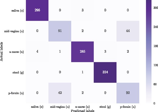
The confusion matrix for the classification of five major body-sites, using Random Forest classifier in a 10×fold cross-validation scheme. The presented body-sites are saliva (o: oral), mid-vagina (u: urogenital), anterior nares (n: nasal), stool (g: gut), and posterior fornix (u: urogenital)

The visualizations of body-site as well as Crohn’s disease samples obtained through using PCA, t-SNE over raw k-mer representations, and t-SNE on the activation function of the last layer of the trained neural networks are presented in Figure 6a and b. These results suggest that supervised training of representations using neural networks provides a non-linear transformation of data that can discriminate between dissimilar environments and host phenotypes.

Fig. 6.

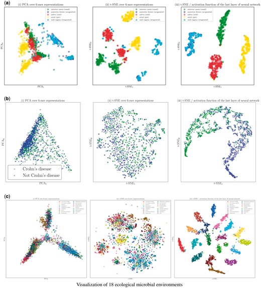
Visualization of (a) body-site, (b) Crohn’s disease, (c) ecological environments datasets using different projection methods: (i) PCA over 6-mer distributions with unsupervised training, (ii) t-SNE over 6-mer distributions with unsupervised training, (iii) visualization of the activation function of the last layer of the trained neural network (projected to 2D using t-SNE). (a) Visualization of the body-site dataset. (b) Visualization of the Crohn’s disease dataset. (c) Visualization of 18 ecological microbial environments

Comparison of k-mer and OTU features in prediction: For a comparison between OTU features and k-mer representations in body-site identification and Crohn’s disease prediction, the RF classifier (as an instance of non-linear classifier) and linear SVM (as an instance of linear classifier) were tuned and evaluated in a stratified 10×fold cross-validation setting. Our results suggest that for both k-mer features and OTUs, RF is the best choice (Table 2). In addition, with almost $\frac{1}{5}$ (body-site dataset) and $\frac{1}{2}$ (Crohn’s disease dataset) of the size of OTU features and in spite of being considerably less expensive to calculate, k-mers marginally outperforms OTU features in both body-site identification and Crohn’s disease classification.

Table 2.

Comparison of k-mers and OTU features in body-site classification as well as the detection of the Crohn’s disease phenotype

Dataset	Features	Classifiers	Micro-metrics (averaged over samples)			Macro-metrics (averaged over classes)
			Precision	Recall	F1	Precision	Recall	F1
Body-site	6-mer features (size: 4096)	RF	0.9 ± 0.03	0.9 ± 0.03	0.9 ± 0.03	0.85 ± 0.04	0.84 ± 0.04	0.84 ± 0.04
		SVM	0.86 ± 0.02	0.86 ± 0.02	0.86 ± 0.02	0.76 ± 0.06	0.76 ± 0.03	0.74 ± 0.04
	OTU features (size: 20 589)	RF	0.89 ± 0.02	0.89 ± 0.02	0.89 ± 0.02	0.83 ± 0.03	0.83 ± 0.03	0.83 ± 0.03
		SVM	0.85 ± 0.03	0.85 ± 0.03	0.85 ± 0.03	0.77 ± 0.05	0.78 ± 0.04	0.76 ± 0.04
Crohn’s disease	6-mer features (size: 4096)	RF	0.76 ± 0.04	0.76 ± 0.04	0.76 ± 0.04	0.76 ± 0.04	0.75 ± 0.04	0.75 ± 0.04
		SVM	0.68 ± 0.04	0.68 ± 0.04	0.68 ± 0.04	0.68 ± 0.04	0.67 ± 0.04	0.67 ± 0.04
	OTU features (size: 9511)	RF	0.74 ± 0.04	0.74 ± 0.04	0.74 ± 0.04	0.74 ± 0.04	0.74 ± 0.04	0.74 ± 0.04
		SVM	0.68 ± 0.04	0.68 ± 0.04	0.68 ± 0.04	0.68 ± 0.04	0.68 ± 0.04	0.68 ± 0.04

Note: For this comparison, Random Forest classifier (as an instance of non-linear classifiers) and linear SVM (as an instance of linear classifiers) have been used. The classifiers are tuned and evaluated in a stratified 10×fold cross-validation setting.

3.2 Ecological and organismal environment prediction

(ii) Classification for different values of k: As stated before, for the ecological and organismal datasets we do not need to perform resampling, as we classify single, representative 16S rRNA sequences for the environment of interest. We thus can skip steps (i) and (iii) (Fig. 3). Step (ii) in Table 3 shows the effect of k in the performance of the classification of the 18 ecological environments for the ECO-18K dataset and 5 organismal environments for 5GUTS-3100. Ecological environments: using k = 6 provides the best classification performance, with a macro-F1 of 0.73 which is relatively high for a 18-way classification (has a mere 0.06 chance of randomly being assigned correctly for balanced dataset). Organismal environments: the results show that k = 6 and 7 provide a high classification macro-F1 of 0.87 for 5 classes (0.2 chance of randomly occurring).

Table 3.

The results for the task of selecting between 18 ecological environments as well as 5 organismal environments belonging to 5 organisms’ gut

Step	Representation	Dataset	Classifier	Micro-metrics (averaged over samples)			Macro-metrics (averaged over classes)
				Precision	Recall	F1	Precision	Recall	F1
(ii)	3-mers	ECO-18K	RF	0.6 ± 0.01	0.6 ± 0.01	0.6 ± 0.01	0.63 ± 0.02	0.6 ± 0.01	0.57 ± 0.01
	4-mers			0.67 ± 0.01	0.67 ± 0.01	0.67 ± 0.01	0.7 ± 0.01	0.67 ± 0.01	0.65 ± 0.01
	5-mers			0.72 ± 0.01	0.72 ± 0.01	0.72 ± 0.01	0.74 ± 0.01	0.72 ± 0.01	0.71 ± 0.01
	6-mers			0.75 ± 0.01	0.75 ± 0.01	0.75 ± 0.01	0.76 ± 0.01	0.75 ± 0.01	0.73 ± 0.01
	7-mers			0.74 ± 0.01	0.74 ± 0.01	0.74 ± 0.01	0.76 ± 0.01	0.74 ± 0.01	0.73 ± 0.01
	8-mers			0.72 ± 0.01	0.72 ± 0.01	0.72 ± 0.01	0.74 ± 0.01	0.72 ± 0.01	0.71 ± 0.01
(ii)	3-mers	5GUTS-3100	RF	0.8 ± 0.02	0.8 ± 0.02	0.8 ± 0.02	0.8 ± 0.02	0.8 ± 0.02	0.79 ± 0.02
	4-mers			0.84 ± 0.01	0.84 ± 0.01	0.84 ± 0.01	0.84 ± 0.01	0.84 ± 0.01	0.83 ± 0.01
	5-mers			0.86 ± 0.02	0.86 ± 0.02	0.86 ± 0.02	0.86 ± 0.02	0.86 ± 0.02	0.85 ± 0.02
	6-mers			0.87 ± 0.01	0.87 ± 0.01	0.87 ± 0.01	0.87 ± 0.01	0.87 ± 0.01	0.87 ± 0.01
	7-mers			0.87 ± 0.01	0.87 ± 0.01	0.87 ± 0.01	0.88 ± 0.02	0.87 ± 0.01	0.87 ± 0.01
	8-mers			0.86 ± 0.01	0.86 ± 0.01	0.86 ± 0.01	0.87 ± 0.01	0.86 ± 0.01	0.86 ± 0.01
(iv)	6-mers	ECO-18K	RF	0.75 ± 0.01	0.75 ± 0.01	0.75 ± 0.01	0.76 ± 0.01	0.75 ± 0.01	0.73 ± 0.01
			SVM	0.79 ± 0.01	0.79 ± 0.01	0.79 ± 0.01	0.79 ± 0.01	0.79 ± 0.01	0.79 ± 0.01
			DNN-3L	0.78 ± 0.01	0.78 ± 0.01	0.78 ± 0.01	0.78 ± 0.01	0.78 ± 0.01	0.78 ± 0.01
(iv)	6-mers	5GUTS-3100	RF	0.87 ± 0.01	0.87 ± 0.01	0.87 ± 0.01	0.87 ± 0.01	0.87 ± 0.01	0.87 ± 0.01
			SVM	0.88 ± 0.02	0.88 ± 0.02	0.88 ± 0.02	0.89 ± 0.01	0.88 ± 0.02	0.88 ± 0.02
			DNN-5L	0.87 ± 0.01	0.87 ± 0.01	0.87 ± 0.01	0.87 ± 0.01	0.87 ± 0.01	0.87 ± 0.01
(iv)	6-mers	ECO-180K	RF	0.83 ± 0.0	0.83 ± 0.0	0.83 ± 0.0	0.84 ± 0.0	0.83 ± 0.0	0.83 ± 0.0
		(10× larger)	SVM	0.86 ± 0.0	0.86 ± 0.0	0.86 ± 0.0	0.87 ± 0.01	0.86 ± 0.0	0.86 ± 0.0
			DNN-5L	0.88 ± 0.0	0.88 ± 0.0	0.88 ± 0.0	0.88 ± 0.0	0.88  ±  0.0	0.88  ±  0.0

Note: The classifiers (Random Forest, Support Vector Machine and neural network classifiers) are tuned and evaluated in a stratified 10×fold cross-validation setting in three datasets ECO-18K, 5GUTS-3100 and ECO-180K. The step column refers to the steps in Figure 3.

(iv) Comparison of classifiers for the selected k: For selected values of k, the results of the environment prediction with the RF, SVM and neural network classifiers are provided [Table 3, step (iv), ECO-18K and 5GUTS-3100 datasets]. The SVM classifier obtained the top macro-F1s of 0.79 and 0.88, respectively for 18-way and 5-way classifications.

To see the effect of increasing the number of data points in classification performance we repeat the classifier comparison (step iv) for the ECO-180K dataset. The results are summarized in Table 3 ECO-18K dataset, showing that feeding more training instances results in better training for the deep learning approach, which outperformed the SVM and achieved a macro-F1 of 0.88, which is very high for a 18-way classification task. In training the neural networks for the ECO-18K dataset, increasing the number of hidden layers from three to more did not help result in improvements. However, using the ECO-180K dataset, which is 10 times larger, allowed us to train a deeper network and increased the macro-F1 by 5% going from 3 layers to 5 layers. Increasing the number of layers further did not result in any improvements.

Neural network visualization: Visualizations of representative 16S rRNA gene sequences in 18 ecological environments obtained through using PCA, t-SNE and t-SNE on the activation function of the last layer of the trained neural network are presented in Figure 6c. For ease of visualization, we randomly picked 100 samples per class. These results suggest that supervised training of representations using neural networks provides a non-linear transformation of data containing information about high-level similarities between environments in the sub-plot on the right [scatter plot (iii)], where such structures appeared in the visualization only when more hidden layers were used: (i) on the left, the environments containing water are clustered in a dense neighborhood: marine, aquatic, freshwater, hot springs, bioreactor sludge (described in the source: ‘Bioreactor sludge is usually the sludge inside the bioreactor that treats waste-water.’), groundwater, and, surprisingly, rhizosphere (an environment where plants, soil, water, micro-organisms and nutrients meet and interact). (ii) In the middle, environments labeled related to sediment are found: sediment, freshwater sediment, marine sediment and soil. (iii) Environments containing food, like food, food fermentation and compost are at the bottom of the plot.

4 Discussion and conclusion

In this work, MicroPheno, a new approach for predicting environments and host phenotypes on 16S rRNA gene sequencing has been presented, which uses k-mer representations of shallow sub-samples. We conclude with discussing the results of this study in three parts: (i) the use of k-mers versus OTUs, (ii) the benefits of shallow sub-sampling and (iii) classical methods versus the deep learning approach.

K-mers versus OTUs: To evaluate MicroPheno, we compared k-mer representations with OTU features in tasks of body-site identification and Crohn’s disease classification. We replicated the state-of-the-art approach, i.e. RF over OTU features, on datasets larger than those that were previously explored. We showed that k-mer features outperform conventional OTUs, while having several advantages over OTUs: (i) The k-mer representations are easy to compute at no computational cost for any type of alignment to references or tasks of finding pair-wise sequence similarity within samples as in OTU-picking pipelines. Just to get an idea of the computational efficiency of k-mer calculation in comparison with OTUs, note that 6-mer distribution calculations have been ≈13 times and ≈20 faster than going through the OTU-picking pipelines respectively for the Crohn’s disease dataset and the Human Microbiome Project dataset; using the same number of threads. More details are provided in the Supplementary Material. (ii) Taxonomy-independent analysis is often the preferred approach for amplicon sequencing when the samples contain unknown taxa. k-mer features can be used without making assumptions about the taxonomy. However, OTU-picking pipelines make assumptions about the taxonomy as discussed in Section 1.2; therefore they can even be phylogenetically incoherent. (iii) The k-mer distribution is a well-defined representation, while OTUs are sensitive to the pipeline and the parameters. (iv) Sequence similarities are naturally incorporated in the k-mer representations for the downstream learning algorithm, while with grouping sequences into certain categories, sequence similarities between OTUs are ignored.

The main disadvantage of k-mer features over OTUs is that using short k-mers makes it more difficult to trace the relevant taxa to the phenotype of interest. When such an analysis is needed, using OTUs or increasing the size of k would be an alternative solution. However, as long as prediction is concerned, using a k-mer representation seems to be the best choice for an accurate and rapid detection/diagnosis over 16S rRNA sequencing samples.

Shallow sub-sampling: We proposed a bootstrapping framework to investigate the consistency and representativeness of k-mer distributions for different sampling rates. Our results suggest that, depending on the k-mer size, even very low sub-sampling rates (0.001 to 0.1, for k between 3 to 7) not only can provide a consistent representation, but can also result in better predictions while possibly avoiding overfitting. Setting aside the saving in preprocessing time as a natural benefit of sampling, this result also suggests that at least for similar phenotypes of interest, shallow sequencing of the microbial community is sufficient for accurate prediction.

Classical classifiers versus deep learning: We studied the use of deep learning methods as well as classic machine learning approaches for distinguishing among human body-sites, diagnosis of Crohn’s disease, and predicting the environments from representative 16S gene sequences. Studying the role of dataset size in the classification of ecological environments showed that for large datasets (in our experiments 10 K samples per class) using deep learning provides us with more accurate predictions. However, when the number of samples is not large enough, RFs performed better on both OTUs and k-mer features. In addition, we observed that for classification over representative sequences as opposed to samples (pool of sequences), the SVM outperformed the RF classifier. Another advantage of using deep learning in classification was that supervised training of a proper representation of data results in a more discriminative representation for the downstream visualization compared to the unsupervised methods (PCA and t-SNE on the raw k-mer distributions). For body-site identification and even more clearly in ecological environment classification, the model was able to extract more high-level similarities between the environments.

Acknowledgements

Fruitful discussions with Andreas Bremges, Till-Robin Lesker, Mohsen Mahdavi, Ali Madani, Yadollah Yaghoobzadeh, Dietmar Pieper, and Marius Vital are gratefully acknowledged.