Association mapping in biomedical time series via statistically significant shapelet mining

Abstract

Motivation

Most modern intensive care units record the physiological and vital signs of patients. These data can be used to extract signatures, commonly known as biomarkers, that help physicians understand the biological complexity of many syndromes. However, most biological biomarkers suffer from either poor predictive performance or weak explanatory power. Recent developments in time series classification focus on discovering shapelets, i.e. subsequences that are most predictive in terms of class membership. Shapelets have the advantage of combining a high predictive performance with an interpretable component—their shape. Currently, most shapelet discovery methods do not rely on statistical tests to verify the significance of individual shapelets. Therefore, identifying associations between the shapelets of physiological biomarkers and patients that exhibit certain phenotypes of interest enables the discovery and subsequent ranking of physiological signatures that are interpretable, statistically validated and accurate predictors of clinical endpoints.

Results

We present a novel and scalable method for scanning time series and identifying discriminative patterns that are statistically significant. The significance of a shapelet is evaluated while considering the problem of multiple hypothesis testing and mitigating it by efficiently pruning untestable shapelet candidates with Tarone’s method. We demonstrate the utility of our method by discovering patterns in three of a patient’s vital signs: heart rate, respiratory rate and systolic blood pressure that are indicators of the severity of a future sepsis event, i.e. an inflammatory response to an infective agent that can lead to organ failure and death, if not treated in time.

Availability and implementation

We make our method and the scripts that are required to reproduce the experiments publicly available at https://github.com/BorgwardtLab/S3M.

Supplementary information

Supplementary data are available at Bioinformatics online.

1 Introduction

Recognizing interpretable patterns that distinguish between cases and controls is instrumental for modern data-driven diagnostics and biomarker discovery (Bellazzi and Zupan, 2008; Wasan et al., 2006). Recent developments in time series classification have focused on discovering shapelets, i.e. subsequences of a time series with high predictive power. Shapelets have already proven useful in various application domains, including genomics (Ghalwash and Obradovic, 2012) and medicine (Ghalwash et al., 2013b), not only because of their competitive classification accuracy, but also because the most discriminative subsequence is straightforward to interpret.

A useful interpretation comes with a high descriptive power, while a good classification accuracy is linked to a high predictive power. However, current shapelet discovery methods do not rely on statistical tests to verify the statistical significance of a shapelet, which makes claims about their interpretability contestable.

We thus propose a new method, S3M (Statistically Significant Shapelet Mining), that returns statistically significant shapelets while maintaining a competitive classification accuracy. The significance of a shapelet is framed as an instance of the multiple hypothesis testing problem, which in turn is mitigated using Tarone’s method (Tarone, 1990). The relevance of S3M is demonstrated by detecting sepsis in time series of the vital signs of intensive care unit (ICU) patients.

1.1 Sepsis

Sepsis is a heterogeneous syndrome that remains a major public health concern due to its association with high mortality, morbidity and health costs (Dellinger et al., 2013; Kaukonen et al., 2014; Peake et al., 2007; Hotchkiss et al., 2016). According to the most recent Sepsis-3 definition, as described by Singer et al. (2016) and Seymour et al. (2016), sepsis is a life-threatening organ dysfunction caused by a dysregulated host response to infection, i.e. a severe reaction to infection driven by physiological and pathological mechanisms.

Up to now, the classification, i.e. distinguishing between patients with sepsis and those without, has proven to be extremely challenging, particularly for patients in the ICU (Raith et al., 2017). If a patient is suspected to suffer from sepsis, one currently determines a broad—and costly—range of clinical and laboratory parameters. In practice, this means that up to 100 individual laboratory parameters are measured per day (Biron et al., 2015; Marshall et al., 2009) because the discovery of a single robust sepsis biomarker is still an open problem.

Clinical parameters are most extensively documented in electronic health records (EHRs) of the ICU. In recent years, several studies have demonstrated the potential of analyzing time series of vital parameters from ICU data (Calvert et al., 2016; Ghalwash et al., 2013a; Shashikumar et al., 2017; Henry et al., 2015). Studying the trajectory of frequently sampled vital parameters, such as the heart rate, solves two challenges at once: (a) taking the temporal signature into account while (b) reducing the need for additional clinical and laboratory parameters.

1.2 Summary

We propose a new statistical association algorithm, S3M, and demonstrate its utility on vital signs of ICU patients with and without sepsis. The contribution of this paper is threefold:

1. Shapelets extracted by S3M guarantee a descriptive power that is supported by a p-value.

2. Our method S3M is scalable and uses only a small set of parameters: the minimum length of a shapelet, the maximum length of shapelet and the desired significance threshold α.

3. Applying S3M to the vital signs of sepsis patients, we discover statistically significant shapelets for diagnosis and biomarker discovery that traditional shapelet discovery methods are unable to identify.

The remainder of this paper is organized as follows: first, Section 2 establishes the theoretical foundations of shapelet discovery methods and statistical pattern mining. Section 2.6 then introduces the new methodology statistical shapelet mining and gives a detailed description of the proposed method S3M. In Section 3, S3M is applied to the vital signs of sepsis patients from the MIMIC-III database (Johnson et al., 2016). Furthermore, we discuss the utility of the proposed method by providing a clear interpretation of the significant shapelets and comparing S3M to traditional shapelet discovery methods. Finally, Section 4 concludes the paper and outlines future research.

2 Statistical shapelet mining

The following sections briefly present some background information on shapelets, their extraction and the significant pattern mining paradigm. Throughout this paper, we assume that we are given a set $\mathcal{T}$ of n time series $\mathcal{T}:=\{T_1$⁠, …, $T_n\}$⁠. Each time series T_i consists of m sequentially ordered measurements, i.e. $T_i:=\{t_{i,1},\dots ,t_{i,m}\}$⁠. Moreover, each time series T_i has an attached class label $y_i\in \{0,1\}$ that denotes the class association (e.g. control versus case).

2.1 Shapelets

Shapelets were introduced by Ye and Keogh (2009) as a new primitive for mining time series. Briefly put, a shapelet is a subsequence of a time series that maximizes predictive power. To obtain shapelets, one uses a sliding window of stride s and width w and extracts all subsequences of a time series, which gives rise to $\lceil (m-w+1)/s\rceil$ subsequences of length w. Every subsequence S (we omit further indices for clarity here) consists of a set of w contiguous positions $\{t_p,\dots ,t_{p+w-1}\}$ of the original time series T, with p satisfying $0\le p\le m-w$⁠. Typically, one uses a stride of s = 1 in time series analysis, meaning that consecutive windows only differ by a single position. We follow this convention here to ensure that no significant shapelets are being missed. Alternatively, one could use a tumbling window approach by setting the stride to be the window width, i.e. s = w, which results in a sequence of non-overlapping windows without any gaps.

Shapelet classification methods require a distance measure for time series $\text{dist}(·)$⁠, usually defined for sequences of the same length. Since shapelets are typically shorter than the original time series, one extends the distance calculation to all subsequences of a time series and finds the minimum of the calculated distances. Formally, given a time series T and a shapelet S, we define

$$\text{dist}(S,T):=\underset{j}{\min }\text{dist}(S,T[j:j+w\left]\right),$$

(1)

where $T[j:j+w]$ refers to the subsequence of length w starting at position j of the time series. The distance between two sequences of equal length, i.e. the term $\text{dist}(S,T[j:j+w\left]\right)$ in the previous equation, is calculated as the standard Euclidean distance (also known as the ${\mathrm{L}}_2$ distance). Using other distance metrics changes the results. Our method thus employs the ${\mathrm{L}}_2$ distance, which is commonly used in the shapelet literature. See Figure 1 for an illustration of the shapelet definition.

2.2 Previous work

The original shapelet classification algorithm, as introduced by Ye and Keogh (2009), uses an iterative procedure to detect suitable shapelets. We briefly recount the algorithm here. First, shapelet candidates are created using the method outlined above. Second, given a candidate shapelet S, its suitability for partitioning all time series is evaluated by means of an information gain criterion. This involves determining the optimal split point of the shapelet with respect to the data, i.e. a distance threshold d_t for which the two classes are best separated. A key observation in finding d_t is that, instead of checking all possible distance thresholds, it is sufficient to check consecutive ones. More precisely, letting $d_0,\dots ,d_{n-1}$ be the sorted distances from S to each of the n time series, one only has to consider thresholds of the form $(d_i+d_{i+1})/2$⁠, as the partition does not change between consecutive distances. Choosing a threshold this way maximizes the separation margin between the two classes.

For each of the candidate thresholds, the information gain is evaluated, and the split point with the best information gain is returned. Ye and Keogh (2009) obtain significant speed-ups by abandoning the calculation of split points early if a shapelet S cannot improve the best information gain that has been identified so far. This is achieved by calculating bounds for the information gain. Further efforts to reduce the computational complexity, such as the technique by Mueen et al. (2011), exploit the reuse of computations as well as caching strategies to speed up the process of selecting suitable shapelets.

As an alternative to these exact methods, various techniques employ heuristics, such as random sampling, to reduce the number of shapelets that have to be considered. Wistuba et al. (2015) present ultra-fast shapelets, which aim to discover relevant shapelets by feature sampling and ranking. The accuracy of this method is shown to be on a par with previous methods, such as fast-shapelets by Rakthanmanon and Keogh (2013). Grabocka et al. (2016) focus on improving run-time performance by clustering similar shapelets during shapelet extraction. Their method does not obtain the best accuracy among all compared algorithms, but is several orders of magnitude faster and permits processing extremely large datasets. An alternative approach is taken by Grabocka et al. (2014), who present an algorithm for learning the relevant shapelets for a given dataset. While this method is shown to yield shapelets with a high predictive power, the large number of parameters makes a direct application unfeasible for now.

2.3 Significant pattern mining

The appeal of shapelet-based approaches is that they yield results that are interpretable and meaningful. At the same time, each of these approaches relies solely on the frequency of a pattern (i.e. a shapelet) to determine its relevance. Especially in the life sciences, however, it is essential to determine whether a detected pattern is also statistically significant within a particular dataset or class. This is the basic premise of significant pattern mining (SPM) algorithms, which have already been successfully employed in itemset mining and subgraph mining tasks (Llinares-López et al., 2015). Recent work by Papaxanthos et al. (2016) demonstrated their applicability in genome-wide association mapping.

Briefly put [see Llinares-López et al. (2015) for a more detailed introduction], SPM algorithms measure the strength of the statistical association using two binary variables, the class variable and the pattern indicator variable, i.e. the variable that indicates whether a pattern occurs in an input. After choosing a test statistic (e.g. Fisher’s exact test) and a corresponding null distribution, the observed value of the test statistic is compared with this null distribution, yielding a p-value. The p-value represents the probability that the test statistic takes a value that is at least as extreme as the observed one. A pattern is deemed significant if this value falls below a certain threshold α. Since the number of patterns is usually extremely large, a ‘naive’ SPM approach is likely to generate a large number of false positives, i.e. patterns that are erroneously considered to be statistically significant. If n_p patterns are being extracted and tested for association, one can expect $\alpha ·n_{\mathrm{p}}$ false positives, even if there are no true associations in the given dataset. Since $n_{\mathrm{p}}\gg n$ in typical applications, an enormous number of false associations will be reported. This is also known as the multiple hypothesis testing problem. One classic way of accounting for multiple testing is controlling the family-wise error rate (FWER), which is the probability of generating one or more false positives, i.e. $\text{FWER}(\delta ):=\mathbb{P}\left(\text{FP}\right(\delta \left)\right)\ge 1$⁠, where $\text{FP}(\delta )$ refers to the number of false positives for a given significance threshold δ. A standard way of controlling the FWER involves the well-known Bonferroni correction (Bonferroni, 1936), which adjusts the significance threshold by dividing it by the number of all detected patterns. We thus get ${\delta }_{\text{bon}}:=\alpha /n_{\mathrm{p}}$⁠. While easy to calculate, this procedure turns out to be extremely conservative, often leading to either no statistically significant patterns, or a severe loss of statistical power. Terada et al. (2013) reported that a statistical advance by Tarone (1990) can be employed instead. This procedure, which we will subsequently expand on, exploits the fact that all involved quantities are discrete, such that only a finite number of p-values can be attained by a pattern. Not only can this insight be exploited to reduce the multiple hypothesis testing burden, it also results in a pruning procedure (which we shall detail below) that speeds up our algorithm while still yielding exact results.

2.4 Significant shapelets

Following the SPM paradigm, our method measures the degree of statistical association between shapelet occurrence and class labels. To obtain a p-value, we need to consider all the different ways in which the shapelet may be used to split the dataset. More precisely, given a candidate shapelet S, we calculate the distances to all time series as described above. This results in a set of distance values $\mathcal{D}:=\{d_1$⁠, …, $d_n\}$⁠. Any distance threshold $\theta \in \mathbb{R}$ results in a partition of the data, i.e. $\mathcal{T}={\mathcal{T}}_{\theta }^{-}\mathrm{\uplus }{\mathcal{T}}_{\theta }^{+}$⁠, where

$${\mathcal{T}}_{\theta }^{-}:=\{T_i\in \mathcal{T}|\text{dist}(T_i,S)\le \theta \},$$

(2)

and ${\mathcal{T}}_{\theta }^{+}$ is defined equivalently. Since the class labels y_i of each time series T_i are known, every choice of threshold gives rise to a contingency table that contains the number of objects associated to a given partition, as well as their class labels (Table 1).

Table 1.

A 2 × 2 contingency table as used by our method

Class label	$\text{dist}(S,T)\le \theta$	$\text{dist}(S,T)>\theta$	Row totals
y = 1	aS	bS	n1
y = 0	dS	cS	n0
Column totals	rS	qS	n

Note: When calculating the minimum attainable p-value for a shapelet, only the values r_S (the number of time series in one part of the partition), n₁ (the number of time series with a positive label), and n (the total number of time series) are required.

2.4.1 Assessing the significance of a shapelet

To determine the best threshold for a given pattern, i.e. the best partition that can be obtained if we use it to split our data, we assess the statistical significance of a given contingency table. The statistical significance is a measure of how likely the given split is if there were no statistical association between the split introduced by the pattern and the data—in other words, assuming that the partition is due to chance. Commonly, statistical significance is achieved by having a p-value (which in turn is obtained by performing a statistical association test) lower than a given significance threshold. The literature knows several association tests, such as Fisher’s exact test (Fisher, 1922), or Pearson’s ${\chi }^2$ test (Pearson, 1900). We use the ${\chi }^2$ test in this paper because it is more appropriate for large sample sizes. Calculating a p-value from a contingency table requires calculating the ${\chi }^2$ test statistic $T_{{\chi }^2}$⁠, which is defined as

$$T_{{\chi }^2}(n,a_S,b_S,c_S,d_S):=\frac{n{(a_S{c}_S-b_S{d}_S)}^2}{(a_S+b_S)(c_S+d_S)(a_S+d_S)(b_S+c_S)}.$$

(3)

From this, we obtain the p-value as

$$1-F_{{\chi }^2}\left(T_{{\chi }^2}(n,a_S,b_S,c_S,d_S)\right),$$

(4)

where $F_{{\chi }^2}(·)$ denotes the cumulative density function of a ${\chi }^2$-distribution with one degree of freedom.

2.4.2 Addressing the multiple hypothesis testing problem

The Bonferroni correction factor t, i.e. the number of tests that we have to account for in shapelet mining, is extremely large, as can be shown by the following calculation. The correction factor t is a product of three quantities, $t=t_1·t_2·t_3$⁠, where:

• $t_1:=n$⁠, the total number of time series in the dataset from which we generate shapelets.

• $t_2:={\sum }_{w=w_{\text{min}}}^{w_{\text{max}}}(m-w+1)$⁠, the number of candidate shapelets per time series, which corresponds to all subsequences of minimum length $w_{\text{min}}$ and maximum length $w_{\text{max}}$⁠.

• $t_3:=n+1$⁠, the total number of candidate split points that we consider.

The Bonferroni-corrected significance threshold per test is therefore:

$$\alpha =\frac{\widehat{\alpha }}{t}=\frac{\widehat{\alpha }}{n(n+1)\left({\sum }_{w=w_{\text{min}}}^{w_{\text{max}}}(m-w+1)\right)}$$

(5)

Hence, even in a rather small dataset with 100 time series of length 100, the number of hypothesis tests is in the order of 10⁶, highlighting the need to improve the statistical power of our approach. One possibility to achieve this improvement is Tarone’s trick (Tarone, 1990).

Tarone (1990) suggested a procedure for discrete test statistics, which allows to gain statistical power when accounting for multiple hypothesis testing. Tarone noted that, as all quantities in the contingency table are discrete, there are only finitely many p-values. In fact, as Terada et al. (2013) show, there is a minimum attainable p-value that only depends on n, n₁ and r_S (the marginal values), but not on the count a_S in the contingency table. The key insight of Tarone (1990) is that if the minimum attainable p-value is larger than the current adjusted significance threshold, a pattern S can never reach statistical significance. Hence, it can also never cause a false positive. Patterns for which this holds are also called untestable hypotheses or untestable patterns. Let n_t denote the number of testable patterns. Then Tarone’s adjusted significance threshold is defined as ${\delta }_{\text{tar}}:=\max \{\delta |\delta ·n_{\mathrm{t}}\le \alpha \}$⁠, which is much larger than ${\delta }_{\text{bon}}$⁠, leading to a gain in statistical power. As the number of testable patterns grows during the extraction process, ${\delta }_{\text{tar}}$ will eventually have to be reduced to ensure that the FWER remains below the desired significance level α. It was shown by Terada et al. (2013) that, owing again to the discrete nature of all the quantities, this reduction only requires us to choose the next relevant p-value from a precalculated set of p-values. We use a closed form for the minimum attainable p-value for fixed n and n₁ (Llinares-López and Borgwardt, 2018). Letting $n_a:=\min (n_1,n-n_1)$ and $n_b:=\max (n_1,n-n_1)$⁠, we have

$$p_{\text{min}}\left(r_S\right):=\{\begin{array}{cc}1-F_{{\chi }^2}\left((n-1)\frac{n_b}{n_a}\frac{r_S}{n-r_S}\right)\hfill & \text{if} 0\le r_S<n_a\hfill \\ 1-F_{{\chi }^2}\left((n-1)\frac{n_a}{n_b}\frac{n-r_S}{r_S}\right)\hfill & \text{if} n_a\le r_S<\frac{n}{2},\hfill \\ 1-F_{{\chi }^2}\left((n-1)\frac{n_a}{n_b}\frac{r_S}{n-r_S}\right)\hfill & \text{if} \frac{n}{2}\le r_S<n_b,\hfill \\ 1-F_{{\chi }^2}\left((n-1)\frac{n_b}{n_a}\frac{n-r_S}{r_S}\right)\hfill & \text{otherwise}.\hfill \end{array}$$

(6)

We can evaluate the preceding equation for $r_S\in \{0,\dots ,n\}$ and store the resulting values in ascending order. They describe all possible values that the adjusted significance threshold ${\delta }_{\text{tar}}$ can attain. Hence, whenever the number of testable patterns is too large to satisfy the desired family-wise error rate, we iterate through the list and choose the largest value for ${\delta }_{\text{tar}}$ such that ${\delta }_{\text{tar}}·n_t\le \alpha$⁠.

2.5 Iterative pruning of shapelet candidates

Tarone’s method only helps us mitigate the multiple hypothesis testing problem. A large amount of time winds up being spent on checking the significance of a given shapelet over all splits. More precisely, given a candidate shapelet S, we need to calculate the distance to every time series, with each distance giving rise to a separate contingency table because the new distance can be used as a threshold for partitioning the data, as described in Section 2.4. However, we are only interested in the p-values associated to significant shapelets. Therefore, we want to abandon processing a candidate shapelet as soon as we are certain that a p-value lower than the current significance threshold ${\delta }_{\text{tar}}$ cannot be obtained. This optimization is based on the insight that since we know how many time series are still to be processed for a partially filled contingency table C with a distance threshold θ, we can bound the p-value that would be achievable under the most extreme circumstances. Such a bound can be obtained by considering two extreme cases:

• Scenario I: we assume that all the remaining time series satisfy $\text{dist}(S,T)\le \theta$ (if their label y = 1) or $\text{dist}(S,T)>\theta$ (if their label y = 0).

• Scenario II: the converse situation, where we assume $\text{dist}(S,T)\le \theta$ for y = 0, and $\text{dist}(S,T)>\theta$ for y = 1.

Formally, we consider a contingency table C to be partially filled whenever $a_S+b_S+c_S+d_S\ne n$⁠, i.e. the sum of its entries does not yet add up to n. Until we have calculated the distance of a shapelet to each time series, every contingency table that we maintain during our algorithm is only partially filled. Since we know that the rows of C sum to n₁ and n₀, we can calculate the number of time series that have not yet been processed by our algorithm as ${\Delta }_1:=n_1-a_S-b_S$ and ${\Delta }_0:=n_0-d_S-c_S$⁠, respectively. We want to abandon the calculation of a partially filled contingency table if its minimum attainable p-value (with ${\Delta }_1$ and ${\Delta }_0$ values still unspecified) is not statistically significant under the current significance threshold ${\delta }_{\text{tar}}$⁠. For this calculation, it is sufficient to consider the ${\chi }^2$ test statistic and show where it attains its maximum values. Using the relations $a_S+b_S=n_1$ and $d_S+c_S=n_0$⁠, we can rewrite the test statistic in terms of a_S and c_S, leading to

$$f_{{\chi }^2}(a,c):=\frac{n{\left(ac-\left(n_1-a\right)\left(n_0-c\right)\right)}^2}{n_1{n}_0(a-c+n_0)(c-a+n_1)}.$$

(7)

The following theorem is the foundation of our pruning strategy.

 

 Theorem 1.

The test statistic $f_{{\chi }^2}(a,c)$ attains its maximum value at the boundary of its domain, i.e.

$$\max \hspace{0.17em}{f}_{{\chi }^2}(a,c):=\underset{a\prime \in [a,a+{\Delta }_1],c\prime \in [c,c+{\Delta }_0]}{\max }{f}_{{\chi }^2}(a\prime ,c\prime )$$

(8)

$$=\max \left(f_{{\chi }^2}(a+{\Delta }_1,c+{\Delta }_0),f_{{\chi }^2}(a,c)\right).$$

(9)

Proof. The test statistic $f_{{\chi }^2}$ is a function of two variables, both of which are defined on a compact domain. Consequently, we know by the multivariate generalization of the extreme value theorem that $f_{{\chi }^2}$ assumes its extreme values either within the domain or on its boundary. We thus calculate the partial derivatives $\partial f_{{\chi }^2}/\partial a$ and $\partial f_{{\chi }^2}/\partial c$ and set them to zero. All solutions are of the form a = t, $c=-(t{n}_0-n_0{n}_1)/n_1$⁠, for $a\in [0,n_1]$⁠. The family of solutions contains the trivial solutions a = 0, c = n₀ as well as a = n₁, c = 0. By analyzing the determinant of the Hessian matrix, we find these solutions to correspond to (local) minima. As a consequence, the function assumes its maximum at the boundary.

Of the four possible boundary cases, it suffices to consider the two cases $a\prime :=a_S+{\Delta }_1,\hspace{0.17em}c\prime :=c_S+{\Delta }_0$⁠, and $a\prime :=a_S,\hspace{0.17em}c\prime :=c_S$⁠, which correspond to the extreme cases of Scenario I and Scenario II as described above. The ‘mixed’ cases that do not fall into any of the two extreme scenarios need not be considered, as the test statistic can always be increased in these cases by decreasing b_S or d_S. □

From the preceding theorem, we know that it is sufficient to consider the two extreme cases mentioned above to calculate two p-values. We denote the minimum of these two values by

$$p_{\text{min}}^{\prime }:=1-F_{{\chi }^2}\left(\max \hspace{0.17em}{f}_{{\chi }^2}(a,c)\right),$$

(10)

because it reflects the possibility that the remaining time series (which we have not seen so far) increase the cell counts in C to lower the p-value maximally. This yields the following decision rule for the iterative pruning of contingency tables: given an incomplete contingency table C with ${\Delta }_1:=n_1-a_S-b_S$ and ${\Delta }_0:=n_0-d_S-c_S$ and

$$p_{\text{min}}^{\prime }>{\delta }_{\text{tar}},$$

(11)

we abandon its calculation because it will never yield a testable shapelet. Hence, we prune the contingency table and will not update it any more when encountering new distances. In case all contingency tables of a shapelet have been pruned because they fail to satisfy testability, we prune the shapelet itself because it can never become testable. In the best case, this criterion thus helps us avoid many (costly) calculations of distances between a shapelet and a time series.

2.6 Significant shapelets with the S3M algorithm

Algorithm 1

S3M (Statistically Significant Shapelet Mining)

Input: Data $\mathcal{D}$⁠, target FWER α

Output: Significant shapelets $\mathcal{S}$⁠, threshold ${\delta }_{\text{tar}}$

1: procedureS3M(⁠$\mathcal{D},\alpha$⁠)

2:  Initialize global${\widehat{\delta }}_{\text{tar}}=1$⁠, global$\widehat{\alpha }\leftarrow 1$⁠, and $\mathcal{S}$ to be empty.

3:   $\mathcal{P}\leftarrow \mathtt{GENERATE}\_\mathtt{ALL}\_\mathtt{MIN}\_\mathtt{P}\_\mathtt{VALUES}$(⁠$\left|\mathcal{D}\right|$⁠)

4:   for subsequence S in $\mathcal{D}$do

5:    $\mathcal{C}$ = $ø$

6:    for Time series $T\in \mathcal{D}$do

7:     UPDATE(⁠$\mathcal{C},\text{dist}(S,T)$⁠)

8:     break if $\mathcal{C}$ is empty

9:    end for

10:    $\mathcal{S},{\delta }_{tar}\leftarrow \mathtt{TARONE}\hspace{0.17em}(\mathcal{P},\mathcal{S},S)$

11:   end for

12:   return$\mathcal{S},{\delta }_{\text{tar}}$

13: end procedure

14:

15: procedureUPDATE(⁠$\mathcal{C}$⁠, d)

16:   Update contingency tables $\mathcal{C}$ with d

17:   for$C\in \mathcal{C}$do

18:    $p_{\text{min}}\leftarrow$BOUNDARY(C)

19:    if$p_{\text{min}}>{\widehat{\delta }}_{\text{tar}}$then

20:     Remove C from $\mathcal{C}$

21:    end if

22:   end for

23: end procedure

24:

25: procedureTARONE(⁠$\mathcal{P},\hspace{0.17em}\mathcal{S}$⁠, S)

26:   $\mathcal{S}\leftarrow \mathcal{S}\cup \left\{S\right\},\hspace{0.17em}\widehat{\alpha }={\widehat{\delta }}_{\text{tar}}·\left|\mathcal{S}\right|$

27:   if$\widehat{\alpha }>\alpha$then

28:    repeat

29:     ${\widehat{\delta }}_{\text{tar}}\leftarrow$ next value from $\mathcal{P}$

30:     Remove untestable patterns from $\mathcal{S}$

31:     $\widehat{\alpha }={\widehat{\delta }}_{\text{tar}}·\left|\mathcal{S}\right|$

32:    until$\widehat{\alpha }\le \alpha$

33:   end if

34:   return$\mathcal{S},\hspace{0.17em}{\widehat{\delta }}_{\text{tar}}$

35: end procedure

36:

37: procedureBOUNDARY(C)

38:   Fill $C_{\text{opt}}$ with remaining $T\in \mathcal{D}$ in a_S and c_S

39:   Fill $C_{\overline{\text{opt}}}$ with remaining $T\in \mathcal{D}$ in b_S and d_S

40:   return min$\{p(C_{\text{opt}}),p(C_{\overline{\text{opt}}})\}$

41: end procedure

42:

43: procedureGENERATE_ALL_MIN_P_VALUES(n)

44:   $\mathcal{P}=ø$

45:   for$r_s\in [0,\dots ,\lfloor \frac{n}{2}\rfloor +1]$do

46:    $\mathcal{P}\leftarrow \mathcal{P}\cup$p_min(r_s) following Equation (6)

47:   end for

48:   Sort $\mathcal{P}$ in descending order

49:   return$\mathcal{P}$

50: end procedure

Algorithm 1 presents our proposed algorithm to discover significant shapelets. This section gives a detailed description of the S3M method and its core subroutines.

First and foremost, the significance threshold ${\widehat{\delta }}_{\text{tar}}$ and $\widehat{\alpha }$ are initialized to 1 and an empty list of significant shapelets and its p-values $\mathcal{S}$ is created. Second, we calculate all possible minimum attainable p-values for the respective dataset. Since for fixed n and n₁$p_{min}\left(r_s\right)$ is symmetric around $n/2$ (Llinares-López and Borgwardt, 2018), we only iterate over half of the possible values r_s can take. Then, the main routine iterates over all subsequences in a sliding window approach to generate the candidate shapelets. For each candidate $S\in \mathcal{S}$⁠, an empty list of contingency tables $\mathcal{C}$ is initialized (Line 5). $\mathcal{C}$ is updated iteratively with the distances dist(S,T) between the candidate S and a time series $T\in \mathcal{D}$ (Line 7). If $\mathcal{C}$ is filled, the list of significant shapelets is updated using the adjusted Tarone threshold (Line 10). Finally, S3M returns the list of significant shapelets and their p-values in $\mathcal{S}$⁠, as well as the adjusted significance threshold ${\widehat{\delta }}_{\text{tar}}$⁠.

The core of the S3M algorithm is the UPDATE routine (Lines 15-23). This routine maintains the list of contingency tables for one candidate shapelet. Assume that k time series have been processed in the outer loop of Line 6. The list of contingency tables $\mathcal{C}$ is then extended by a new contingency table corresponding to the new split point (θ_k) introduced by the distance to the candidate shapelet S. All remaining contingency tables C_i with thresholds θ_i are also updated. Line 17 iterates over all tables in $\mathcal{C}$ and computes the minimum possible p-value according to Theorem 1 (Line 18; see subroutine BOUNDARY). If the minimum possible p-value exceeds the Tarone threshold, the corresponding table is untestable and thus removed from the list. Finally, if $\mathcal{C}$⁠, the list of contingency tables, is empty in Line 8, the pruning criterion sets in: regardless of the remaining time series, shapelet S cannot be significant and thus the for loop of Line 6 breaks and the next candidate shapelet will be considered.

The subroutine TARONE in Lines 25-35 maintains the list of significant shapelets $\mathcal{S}$ and adjusts the Tarone threshold ${\widehat{\delta }}_{\text{tar}}$⁠. In each iteration, ${\widehat{\delta }}_{\text{tar}}$ is lowered such that untestable patterns according to Tarone are excluded. This routine is conceptually similar to Lines 18-28 of Algorithm 1 in Llinares-López et al. (2015) and follows the multiple testing correction described in Section 2.4.2. Please note that TARONE will perform no operation if the list of contingency tables $\mathcal{C}$ is empty.

Finally, the subroutine BOUNDARY implements Theorem 1 in that it returns the minimum p-value $p_{\text{min}}^{\prime }$ of the two extreme cases given a partially filled contingency table C. This routine has two important properties: first, $C_{\text{opt}}$ and $C_{\overline{\text{opt}}}$ are unique, given n and n₁ as in Table 1. Second, the routine for computing the p-value in Line 40 is modular. Here, we use the ${\chi }^2$ test because it is better suited for larger sample sizes than Fisher’s exact test. However, Fisher’s exact test yielded similar results in our experiments.

3 Experiments

The performance of statistically significant shapelet mining is assessed on real-world data from sepsis patients. First, the MIMIC-III database, how sepsis cases and controls are extracted, and the evaluation settings are described. A brief comparison of the results of the proposed method (S3M) and a state-of-the-art comparison partner (gRSF) follows. Finally, the statistically most significant shapelets are interpreted and discussed.

3.1 Experimental setup

Our analysis is based on version 1.4 of the MIMIC-III (Multiparameter Intelligent Monitoring in Intensive Care) database (Johnson et al., 2016). It includes over 45 000 de-identified critical care patients and data from over 50 000 ICU stays. We base our queries on examples from the MIMIC code repository [Johnson et al. (2018), see public repository], to extract the vital signs of 355 ICU stays that resulted in sepsis episodes from 352 individual patients. We limit the application of our algorithm to heart rate, respiratory rate, and systolic blood pressure, because these parameters are routinely measured in ICU stays for monitoring a patient’s stability, but also play an important role in the assessment of sepsis-related organ failure; see for example the qSOFA score (Singer et al., 2016).

3.1.1 Preprocessing

For the sepsis cases, we consider patients for which both of the following two criteria are met:

1. A suspected infection (SI) that started later than four hours after admission to the ICU and before ICU discharge. The SI criterion manifests in antibiotic administration and sampling of body fluid cultures.

2. An increase of two points of the SOFA score (Vincent et al., 1996) around the time of SI, comparing the maximum of two time frames: One between five to two days before SI, the other between two days before to one day after SI.

These two conditions are adapted from the definition of Seymour et al. (2016), which was employed in a retrospective study design for the assessment of clinical criteria for sepsis.

The control cohort consists of all ICU episodes during which no sepsis was encountered. Note that the set of controls may therefore include edge cases that meet only one of the two criteria including patients whose sepsis episode was before or immediately after the ICU stay. Defining an exhaustive control group makes the task more challenging but also more realistic. In contrast, a more restrictive case-control selection, neglecting edge cases, would tend to overestimate the classification accuracy.

The experimental setup requires additional filtering of the raw MIMIC-III database: First, patients that fall below the age of 15 and patients where no chart values were available, are excluded. Second, patients where ICU stays are logged via the CareVue system are excluded, because CareVue underreports negative microbiology lab values that are essential to the Sepsis-3 definition [for details, see Desautels et al. (2016)]. Third, in order to not extract most shapelets from few very long ICU stays, we restricted our analysis to only consider the first 75 hours. Fourth, to ensure pairwise comparability, we used forward filling and backward filling to upsample aperiodically reported vital signs to a rate of 30 minutes. Finally, to balance the dataset, we downsampled the 21 079 (34.26%) controls to the number of cases (355, 0.58%).

Applying these criteria to all 61 195 ICU stays, the resulting cohort consisted of 355 cases and 355 controls. Please refer to our public repository that provides additional details about the method, the data and how to reproduce the results.

3.1.2 Parameters

In the following, we use S3M to extract shapelets of length 4-6 resulting in subsequences that range from two hours to three hours. Longer window sizes are possible but may not be useful in a diagnostic setting, according to our domain experts. We enforced a significance level of $\widehat{\alpha }=0.01$⁠. Furthermore, we only consider a random sample (containing 75 cases and 75 controls) of the systolic blood pressure data because the time series are not sufficiently distinct from each other, resulting in many shapelets that are virtually identical and do not offer more insight.

3.1.3 Comparison baseline

Since our method is the first shapelet-based method that employs a statistical measure, there are no canonical comparison partners. We thus select a recent and very strong (in terms of predictive performance) baseline algorithm, namely generalized random shapelet forests (gRSF) (Karlsson et al., 2016), and assess its statistical performance in a post-processing step: for each shapelet S returned by the baseline algorithm, we compute its p-value p_S using the ${\chi }^2$ test on the contingency table of the test set. We then follow the decision rule $p_S<\alpha$ for assessing the statistical significance of the shapelet, where $\alpha :=\widehat{\alpha }/\#\text{Candidates}$ extends the significance threshold from Equation (5) by the number of candidates that have been considered. Note that the additional Bonferroni correction needs to be employed for all possible candidates, even if some have been pruned, because they are still tested implicitly.

3.1.4 Evaluation

In every experiment, we divided the 355 cases and 355 controls into a training and test set with a ratio of 2:1. The performance of existing shapelet-based methods is typically measured in terms of accuracy or similar classification metrics. While these metrics are commonly used to evaluate predictive performance, they do not necessarily yield insights into the descriptive power of the features or shapelets. Hence, we also evaluate the statistical significance, namely the p-value of the extracted shapelets. As we shall see below, existing methods do not discover statistically significant patterns because they do not take into account the multiple hypothesis testing problem.

3.2 Results

Table 2 summarizes the number of detected significant shapelets and shows that our proposed S3M method identifies a plethora of statistically significant shapelets for all considered vital signs whereas the comparison baseline detects none.

Table 2.

Number of statistically significant shapelets after adjusting for multiple hypothesis testing

Vital sign	S3M	${\delta }_{\text{tar}}$	gRSF	α
Heart rate	200	2.51 × 10−10	0	1.28 × 10−15
Respiratory rate	514	4.47 × 10−10	0	1.33 × 10−15
Systolic blood pressure	58	2.55 × 10−9	0	4.35 × 10−14

Note: Our proposed method S3M returns many significant shapelets, in contrast to the baseline competitor gRSF, which does not yield any significant shapelets. We denote the significance threshold reached by our method as ${\delta }_{\text{tar}}$⁠, and the Bonferroni correction factor by α.

Prior to describing the individual shapelets, we first give an overview of all the shapelets detected by our method. We use the heart rate dataset as an example; refer to Supplementary Figures S1 and S2 for the remaining datasets. Following the terminology of Section 2.6, we visualize the contingency table corresponding to the best p-value of a candidate shapelet. Being represented by its counts a_S, b_S, c_S, and d_S, we map each table to the coordinates $x_1=(a_S-b_S)/(a_S+b_S)$ and $x_0=(c_S-d_S)/(c_S+d_S)$⁠. The x₁ coordinate thus measures the presence of the shapelet in cases (y = 1), while the x₀ coordinate measures its absence in controls (y = 0). In an ideal scenario, $(x_1,x_0)\approx (1,1)$ would imply that $a_S\gg b_S$ and $c_S\gg d_S$⁠, i.e. the shapelet occurred in cases while being absent in controls. Figure 2 depicts the contingency tables of all candidate shapelets (gray) in the heart rate dataset. We observe that the subset of statistically significant shapelets (red) is distinctly scattered in the upper-right part of the visualization. This implies that they are predominantly present in cases and absent in controls. Similar results hold for the remaining datasets. The contingency tables of the statistically most significant shapelet in each dataset (Table 3) also exhibit this property; in every table, the counts satisfy $a_S\gg b_S$ and $c_S\gg d_S$⁠.

Table 3.

The contingency tables of the statistically most significant shapelets identified by S3M for the three datasets

$$[\begin{array}{cc}163& 74\\ 69& 168\end{array}]$$	$$[\begin{array}{cc}154& 83\\ 55& 182\end{array}]$$	$$[\begin{array}{cc}71& 4\\ 29& 46\end{array}]$$
(a) Heart rate	(b) Respiratory rate	(c) Systolic blood pressure

Note: Each table follows the notation from Table 1, i.e. a_S, b_S in the top and d_S, c_S in the bottom row.

Fig. 1.

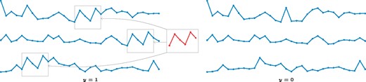
Schematic illustration of a shapelet, a time series motif, and its occurrences in a data set of time series that belong to one of two phenotypic classes (left: y = 1, right: y = 0). The shapelet is enriched in one class (y = 1). Note that the decision whether a shapelet occurs depends on a distance threshold

Interestingly, when we randomly permute the labels of our time series (Supplementary Fig. S3), we observe that (i) our method does not detect any statistically significant shapelets, which gives additional credibility to the shapelets that we identified in the nonpermuted data, and (ii) all candidate shapelets in the visualization move closer to the dashed line (meaning that they are more weakly associated with the class labels), and start to appear on both sides of the line (meaning that some shapelets are associated with supposed controls as well).

Next, we focus only on the statistically most significant shapelet (i.e. among the significant shapelets, the one with the lowest p-value on the test set), in order to discuss the biomedical insights our shapelets reveal. Figure 3 depicts the statistically most significant shapelets of the three datasets within the context of the time series they originated from, along with their p-value on the test dataset. Prior to addressing the biomedical relevance of our shapelets, we briefly assess their predictive accuracy on the test dataset. Table 4 shows that the accuracy of a single shapelet (the statistically most significant one) is comparable to the baseline method (gRSF), which employs over 3000 statistically insignificant shapelets. We hence observe that the use of statistically significant shapelets may also result in a competitive classification accuracy.

Table 4.

Classification accuracy of S3M versus gRSF (average out of 10 repetitions) on the test set

Vital sign	S3M	# Shapelets	gRSF	# Shapelets
Heart rate	0.70	1	0.74	3030
Respiratory rate	0.71	1	0.76	3406
Systolic blood pressure	0.75	1	0.74	971

Bold values are used to highlight the best predictive performance (accuracy) of the compared methods. Note: The proposed S3M method only uses one shapelet, whereas gRSF constructs a decision tree based on multiple shapelets.

Fig. 2.

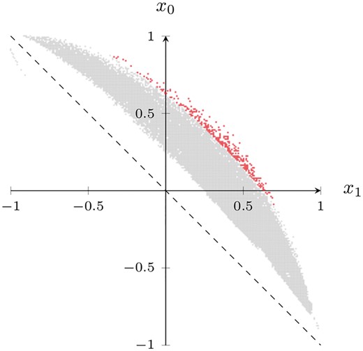
Following Section 3.2, we generate the coordinates from the contingency table of each shapelet such that the axes represent a relative measure of the degree to which a shapelet is present in cases (x₁) and absent in controls (x₀). This results in a point cloud of all shapelets (gray). The statistically significant shapelets (red) identified by the proposed S3M method form a distinct subset. Their coordinates indicate that they are predominantly present in cases and absent in controls

Fig. 3.

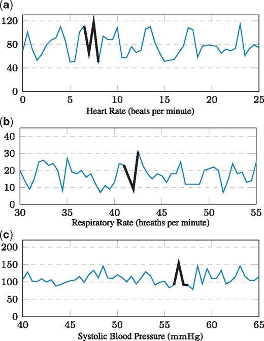
The three most statistically significant shapelets that our algorithm extracted for the three datasets (a-c). Each shapelet is shown within the context of the time series it is extracted from. The x-axis depicts the hour since ICU admission

3.3 Medical interpretation of the most significant shapelets

Univariate time series of three vital signs (heart rate, respiratory rate and systolic blood pressure) in septic and non-septic ICU patients have been analyzed using the proposed S3M algorithm. S3M extracts a set of statistically significant shapelets for each of the datasets.

First, observing the shapelets in the visualization (Fig. 2) are mostly present in the first quadrant (upper-right corner) as opposed to the third one (lower-left corner), our conjecture is that the span of the shapelet search space is different for cases and controls.

Second, many previous EHR analyses distinguish themselves by reporting predictive accuracies. However, statistically more elaborate approaches too often are being evaluated by predictive scoring alone which might hinder interpretability and deeper domain-specific insight. In the following, we discuss how statistically significant shapelets help obtain insights into biomedical time series by providing interpretable and statistically significant patterns.

Figure 3a depicts the most significant heart rate shapelet. A comparison with Table 3a shows that this episode of transient instability predominantly occurred in case time series. Since this observation appears to contradict recent findings on heart rate variability—which is supposed to decrease with increasing sepsis severity (de Castilho et al., 2017; Ahmad et al., 2009)— further elaborate on it: the common notion of heart rate variability (HRV) is crucially different from our setting. HRV is defined as a measure of varying inter-beat (RR) intervals in the electrocardiogram (ECG). Typically, it is measured in sub-second resolution over long time periods. By contrast, we study heart rate frequency, i.e. beats per minute, with a sampling frequency of 30 minutes. Moreover, the proposed approach identifies significant localized episodes of heart rate variation (occurring within a period of few hours), whereas ECG summary statistics fail to capture them. While conventional HRV (measured every second on a high-frequency scale) can indicate healthy autonomic regulation, our findings suggest that episodes of low-frequency variability (measured every 30 minutes and observed over few hours) could be relevant for sepsis, for instance as a sign of sudden hemodynamic instability. This suggests that the S3M method is able to capture and reveal pathophysiologically relevant mechanisms.

Figure 3b depicts the result for respiratory rate. It is already well established that several septic pathomechanisms lead to an increased respiratory rate (e.g. lactate acidosis, pulmonary edema, damaged respiratory center). However, in this plot, the statistically most significant respiratory rate shapelet tends to exploit a sudden transient drop to a low absolute level. Table 3b, the corresponding contingency table, shows that the pattern is associated with cases. Interestingly, such a pattern is independent of the established understanding of increased respiratory rate in septic patients.

Finally, Figure 3c shows the most significant systolic blood pressure shapelet. Here, the shapelet does not merely distinguish between higher and lower levels of blood pressure (associated with circulatory failure), but rather constitutes a specifically shaped, predictive spike, which is statistically significantly enriched in case time series (Table 3c).

These insights still remain in the hypothesis-generating realm and require further investigation. Nevertheless, they demonstrate the utility of our method for the analysis of challenging biomedical datasets: using a computationally efficient and statistically sound approach, our S3M method is able to automatically retrieve statistically significant, predictive, and interpretable patterns that permit a deeper understanding of a high-impact clinical field.

4 Conclusion

In this work, we have introduced a scalable method for the identification of statistically significant patterns in biomedical time series. The proposed S3M methodology uses shapelets (short subsequences of a time series) and assesses their statistical significance by means of association testing. We employ a statistical method introduced by Tarone (1990) to mitigate the multiple hypothesis testing problem and to improve the run-time by pruning untestable shapelets. In the experimental part of this work, we analyzed time series of vital signs of patients suffering from sepsis. We demonstrated the biomedical relevance of shapelets extracted from the heart rate, the respiratory rate, and the systolic blood pressure, which state-of-the-art competing methods are unable to identify.

The concept of statistically significant shapelets results in patterns that (i) have a meaningful interpretation, and (ii) are computationally efficient to obtain. In contrast, in the traditional setting, none of the shapelets are deemed statistically significant due to a lack of statistical power. We also showed how a modification of the ideas of Tarone (1990) can be used to yield additional computational advantages when considering contingency tables that are only partially filled. In many cases, this permits our algorithm to skip a large part of the search space without sacrificing its exactness.

Given the competitive predictive performance of the identified patterns, post-processing of significant shapelets will be an exciting route for future research. A next step could involve their clustering. In this context, the statistical significance of our patterns helps avoid the issues with clustering subsequences, as outlined by Keogh and Lin (2005). Moreover, the significant shapelets we discovered in sepsis patients have a clear medical interpretation. This demonstrates that statistically significant shapelet mining can also be employed for diagnostic purposes and biomarker discovery in future work.

Funding

KB acknowledges funding from the SNSF Starting Grant “Significant Pattern Mining” and the SPHN/PHRT Driver Project “Personalized Swiss Sepsis Study”.

Conflict of Interest: none declared.