Finding associated variants in genome-wide association studies on multiple traits

Abstract

Motivation

Many variants identified by genome-wide association studies (GWAS) have been found to affect multiple traits, either directly or through shared pathways. There is currently a wealth of GWAS data collected in numerous phenotypes, and analyzing multiple traits at once can increase power to detect shared variant effects. However, traditional meta-analysis methods are not suitable for combining studies on different traits. When applied to dissimilar studies, these meta-analysis methods can be underpowered compared to univariate analysis. The degree to which traits share variant effects is often not known, and the vast majority of GWAS meta-analysis only consider one trait at a time.

Results

Here, we present a flexible method for finding associated variants from GWAS summary statistics for multiple traits. Our method estimates the degree of shared effects between traits from the data. Using simulations, we show that our method properly controls the false positive rate and increases power when an effect is present in a subset of traits. We then apply our method to the North Finland Birth Cohort and UK Biobank datasets using a variety of metabolic traits and discover novel loci.

Availability and implementation

Our source code is available at https://github.com/lgai/CONFIT.

Supplementary information

Supplementary data are available at Bioinformatics online.

1 Introduction

Over the past few decades, genome wide association studies (GWAS) have found numerous genetic variants associated with phenotypic variation (Dorn and Cresci, 2009; Eskin, 2015; McCarthy et al., 2008). These phenotypes include a wide range of diseases and medically relevant traits such as heart disease (Dorn and Cresci, 2009; Lee et al., 2013; Nikpay et al., 2015), cholesterol level (Postmus et al., 2016) and depression (Cai et al., 2015; Hyde et al., 2016), among others. In some cases, variants have been found to affect multiple traits, a phenomenon known as pleiotropy (Andreassen et al., 2015). For example, multiple psychiatric disorders, immune diseases and nervous system phenotypes have been found to share causal variants (Chen et al., 2016; Chesler et al., 2005; Cross-Disorder Group of the Psychiatric Genomics Consortium, 2013; Solovieff et al., 2013; Zeggini and Ioannidis, 2009). Variants associated with disease have also been found to be associated with tissue-specific gene expression phenotypes (Liu et al., 2016). Considering multiple traits at once may increase power to detect variant effects when there is pleiotropy.

One approach to combine information from different studies is to apply meta-analysis. Meta-analysis methods are often used in GWAS to combine results from different studies on the same trait to increase power (Berndt et al., 2016; Nikpay et al., 2015; Postmus et al., 2016). Intuitively, one can effectively increase the sample size by pooling summary statistics from multiple small studies, which also have the benefit of being more readily obtainable compared to individual level data. The two classic versions of meta-analysis are fixed effects (FE) meta-analysis and random effects (RE) meta-analysis (Fleiss, 1993). In the FE model, a variant is assumed to have the same effect in each study, which is only realistic if all studies in the meta-analysis measure the same phenotype in the same population. If instead the true effect size differs between studies, we say there is heterogeneity. The RE model allows for heterogeneity by assuming study-specific effect sizes are drawn independently from a normal distribution. The binary effects (BE) model also allows for heterogeneity (Han and Eskin, 2012). In BE meta-analysis, a variant may either have an effect of fixed size or no effect in each study (Han and Eskin, 2012). A variant’s configuration of effects across traits may then be expressed as binary vector with entries indicating whether or not the effect is zero for each trait.

However, it is problematic to directly apply meta-analysis to combine studies that analyze different traits for a number of reasons. First, some traits share many causal variants while others share very few. Existing meta-analysis methods do not allow for varying degrees of shared variants between traits, and combining unrelated traits in a meta-analysis may actually decrease power compared to independent analysis of such traits. Second, a variant that affects one trait may have no effect in a different trait. While RE meta-analysis and related methods allow for differences in effect size between studies, such methods inherently assume an effect is present in all studies in the meta-analysis. Finally, studies may share individuals across traits. For example, data on several traits may be collected from the same cohort of individuals. Meta-analysis techniques assume that the studies are independent, but this only holds if the studies are performed on non-overlapping individuals.

In this paper, we present CONFIT, a novel meta-analysis method for multiple traits that addresses these shortcomings. CONFIT estimates the degree of shared effects between traits from the data using GWAS summary statistics, then uses these estimates to analyze multiple traits while allowing effects to be present in only a subset of the traits. CONFIT is inspired by the existence of pleiotropy and its potential to increase power to detect variants that affect multiple traits. Unlike traditional meta-analysis methods, CONFIT is designed to combine GWAS on different traits and does not assume a particular relationship between the different traits. Our test statistic is a likelihood ratio averaged over many models, where each model assumes the variant to have non-zero effect in a particular subset of traits and is weighted by a prior estimated from the data.

We tested CONFIT and show it has increased power compared to multiple independent (MI) GWAS in simulated data when variants have effect in multiple traits. We also show CONFIT accounts for correlated effect size estimates from overlapping individuals between studies. We then demonstrate that CONFIT finds unique loci when combining studies on multiple traits using the North Finland Birth Cohort (NFBC) dataset and the UK Biobank (UKKB) dataset. CONFIT has many potential applications due to the vast variety of GWAS datasets available.

2 Materials and methods

2.1 Finding associated variants in one trait using a genome-wide association study (GWAS)

We now describe how to test a variant v for association in a trait t using a GWAS. Let ${\mathbf{g}}_{vt}$ be the vector of genotype values in n_t individuals collected in the study for trait t. Denote entry j in ${\mathbf{g}}_{vt}$ as $g_{vt,j}$⁠, which corresponds to the genotype of the jth individual in study t, i.e. the number of copies of variant v they possess. Thus $g_{vt,j}\in \{0,1,2\}$⁠. Let ${\mathbf{x}}_{vt}$ be the vector of standardized genotype values in study t. In other words, ${\mathbf{x}}_{vt}$ is obtained by mean-centering and scaling ${\mathbf{g}}_{vt}$ to have a sample variance of 1.

Let ${\mathbf{y}}_t$ be the vector of phenotype values in n_t individuals for trait t. Assume ${\mathbf{y}}_t$ has been centered to have mean 0. Given ${\mathbf{x}}_{vt},{\mathbf{y}}_t$⁠, GWAS assumes the linear model

$${\mathbf{y}}_t={\beta }_{vt}{\mathbf{x}}_{vt}+{\mathbf{e}}_t$$

(1)

where β_vt is the effect of v on trait t and ${\mathbf{e}}_t\sim N(0,{\sigma }_e^2\mathbf{I})$ is gaussian noise (Eskin, 2015). The magnitude of β_vt indicates how predictive v is. One then finds the estimated effect ${\widehat{\beta }}_{vt}$ by linear regression. The solution given by ordinary least squares is

$${\widehat{\beta }}_{vt}={({\mathbf{x}}_{vt}^{\mathrm{⊺}}{\mathbf{x}}_{vt})}^{-1}{\mathbf{x}}_{vt}^{\mathrm{⊺}}{\mathbf{y}}_k$$

(2)

where

$${\widehat{\beta }}_{vt}\sim N({\beta }_{vt},{({\mathbf{x}}_{vt}^{\mathrm{⊺}}{\mathbf{x}}_{vt})}^{-1}{\sigma }_e^2)$$

(3)

Since ${\sigma }_e^2$ is unknown, we estimate it as ${\widehat{\sigma }}_e^2=\frac{1}{n_t-1}\left|\right|{\mathbf{y}}_t-{\widehat{\beta }}_{vt}{\mathbf{x}}_{vt}|{|}_2^{\mathrm{2}}$⁠. Let $d_{vt}={({\mathbf{x}}_{vt}^{\mathrm{⊺}}{\mathbf{x}}_{vt})}^{-1}{\widehat{\sigma }}_e^2$⁠. The summary statistic for v in study t is then the pair $({\widehat{\beta }}_{vt},d_{vt})$⁠. One may also estimate ${\widehat{\beta }}_{vt}$ and d_vt using a LMM, which corrects for population structure within the study cohort (Furlotte and Eskin, 2015; Kang et al., 2010).

Because the variance may differ from study to study, we normalize each effect by its standard error to obtain a z-score, where for each variant v, we have

$$z_{vt}={\widehat{\beta }}_{vt}/\sqrt{d_{vt}}\sim N({\lambda }_{vt},1)$$

(4)

where λ_vt is the true normalized effect size. One may then use z_vt as a test statistic to test whether v is associated with t. Let α be the desired significance level. If $\left|z_{vt}\right|$ exceeds some threshold value $z_{\alpha }$⁠, or equivalently, $p(z_{vt})=\mathrm{Pr}(|z|\ge |z_{vt}|\hspace{0.17em}|H_0)\le \alpha$⁠, then we conclude v is significantly associated with t.

Because a typical GWAS may test millions of variants, α should be set to account for multiple testing at the variant level. Say 0.05 is the desired significance level for the whole family of tests. A simple way to correct for multiple testing is to apply the Bonferroni correction, which yields $\alpha =0.05/\left|V\right|$⁠. However, due to the presence of linkage disequilibrium (LD) in the human genome, the Bonferroni correction on the total number of variants is overly conservative. In the GWAS community, α_GWAS = 5× 10^–8 is commonly accepted as a significance level that takes into account the number of SNPs and presence of LD in the human genome (Consortium, 2005; McCarthy et al., 2008; Pe’er et al., 2008).

2.2 Finding associated variants in at least one of multiple traits using MI GWAS

Suppose we have a variant v and a set of traits $T=\{t_1,\dots ,t_k\}$⁠, and we are given GWAS effect sizes and variance (⁠${\widehat{\beta }}_{vt},d_{vt}^2$⁠) of v for each trait t in T. To perform MI GWAS on a set of traits, one simply performs a GWAS as described above for each variant v on each trait to obtain a vector of z-scores across traits $\mathbf{z}={(z_{v{t}_1},z_{v{t}_2},\dots ,z_{v{t}_k})}^{\mathrm{\top }}$⁠. The MI GWAS test statistic is then ${\max }_t\left|z_{vt}\right|$⁠, or equivalently the smallest GWAS P-value across traits, ${\min }_t\hspace{0.17em}p(z_{vt})$⁠. In MI GWAS, one must correct for two levels of multiple testing–multiple variants and multiple traits. If we assume each trait to be an independent test, then we may apply Bonferroni correction for k traits to α_GWAS, yielding multiple testing corrected significance level α_MI = α_GWAS/k. Then v is significant if min_t p(z_vt) ≤ α_MI.

2.3 Finding associated variants using CONFIT

CONFIT attempts to find variants $v\in V$ that affect at least one of k traits $t_1,\dots ,t_k$⁠, given summary statistics from a GWAS on each trait. CONFIT assumes each variant v either has zero effect on the trait, or if it has non-zero effect, that its normalized effect size, i.e. its NCP, follows a Fisher polygenic model. We describe whether the variant has non-zero effect in each of the k traits using a binary vector $\mathbf{c}={[c_1\dots c_k]}^{\mathrm{⊺}}$⁠, where c_t = 1 if the variant is active in trait t in that configuration and 0 otherwise.

For convenience, we use a fixed λ for all traits and variants when explaining the test statistic in this section. This fixed λ assumption is very strong. Later, we describe how this assumption can be relaxed to allow different NCPs for each variant v. We also assume the z-scores are independent across studies given the activity configuration, but will also relax this assumption in a later section. Let ${\mathbf{z}}_v={[z_{v{t}_1},\dots ,z_{v{t}_k}]}^{\mathrm{\top }}$ Then

$${\mathbf{z}}_v\sim N(\lambda \mathbf{c},\mathbf{I})$$

(5)

Our test statistic at v is a likelihood ratio with multiple alternate models, where model is a different activity configuration. The statistic has the likelihoods of each alternate configuration against ${\mathbf{c}}_0$⁠, weighted by a prior on each configuration $\mathrm{Pr}(\mathbf{c})$⁠. Let C denote the set of all possible configurations and ${\mathbf{c}}_0$ denote the null configuration ${\mathbf{c}}_0={[0\dots 0]}^{\mathrm{⊺}}$⁠, and C_A denote the set of alternate configurations, $C_A=C\mathrm{\setminus }\left\{{\mathbf{c}}_0\right\}$⁠. Then

$$F_v=\sum _{\mathbf{c}\in C_A}\frac{\mathrm{p}(\mathbf{z}|\mathbf{c},\lambda )\mathrm{Pr}(\mathbf{c})}{\mathrm{p}(\mathbf{z}|{\mathbf{c}}_0)\mathrm{Pr}({\mathbf{c}}_0)}\hspace{0.17em}$$

(6)

2.4 Setting a prior on each activity configuration

Many choices of prior on the configurations are possible. We set an initial prior $\underset{0}{\mathrm{Pr}}(\mathbf{c})$ as the fraction of variants which have univariate GWAS P-value less than threshold ${10}^{-4}$ in the subset of traits that are active in $\mathbf{c}$⁠. We chose ${10}^{-4}$ as a threshold because we wished to capture shared effects between variants which are not necessarily strong enough to reach GWAS significance. If $\mathbf{c}$ contains only one active trait, we set the final prior $\mathrm{Pr}(\mathbf{c})$ by averaging $\underset{0}{\mathrm{Pr}}(\mathbf{c}\prime )$ over all configurations $\mathbf{c}\prime$ with a single active trait. Otherwise we set $\mathrm{Pr}(\mathbf{c})=\underset{0}{\mathrm{Pr}}(\mathbf{c})$⁠. The reason for this is that the CONFIT model assumes a similar distribution of GWAS z-scores for each trait, but in real life, some traits may tend to have larger effects and others to have smaller effects. We mitigate this by averaging the prior for each trait alone being active. Then traits with large effect sizes will still have high power even with a smaller prior on their configuration, and traits with small effect sizes will now have a power boost with a larger prior. This is the default choice of prior for CONFIT.

2.5 Significance testing with ${\mathrm{F}}_v$

We now describe how to find a P-value and perform significance testing for variant v using ${\mathrm{F}}_v$⁠.

We find a null distribution for ${\mathrm{F}}_v$ by generating GWAS summary statistics at a variant v under the null hypothesis, by drawing vector of z-scores for each trait $\mathbf{z}\sim N(0,I)$⁠. To generate GWAS summary statistics under the null in the real dataset, one may permute the labels on the set of phenotypes for each trait, such that the correlation between traits is preserved but variant-phenotype correlation is not before performing GWAS, or one could perform GWAS on the real genotypes and simulated phenotypes generated under the null.

The null distribution of ${\mathrm{F}}_v$ also depends on the estimated priors $\{\mathrm{Pr}(\mathbf{c}):\mathbf{c}\in C\}$⁠. Say we have estimated priors $\{\mathrm{Pr}(\mathbf{c}):\mathbf{c}\in C\}$ from the data. We generate GWAS summary statistics for $5\times {10}^9$ variants under the null hypothesis and compute ${\mathrm{F}}_v$ on the null data using the $\{\mathrm{Pr}(\mathbf{c}):\mathbf{c}\in C\}$ from the original data. Then we have obtained a null distribution for ${\mathrm{F}}_v$⁠. The P-value of ${\mathrm{F}}_v,\hspace{0.17em}p({\mathrm{F}}_v)$ is the fraction of null variants with test statistic less than ${\mathrm{F}}_v$⁠. Let $p_{\alpha }$ be the desired P-value threshold. If $p({\mathrm{F}}_v)\le p_{\alpha }$⁠, we then conclude variant v is associated with at least one of the k traits.

In a simulated dataset containing m independent variants, one may set $p_{\alpha }$ as the Bonferroni corrected threshold $p_{\alpha }=0.05/m$⁠. However, the Bonferroni correction is overly stringent when LD is present between variants, as is the case in real datasets. For the NFBC and UKBB datasets, we perform significance testing with ${\mathrm{F}}_v$ at the P-value threshold $p_{\alpha }=5\times {10}^{-8}$⁠. This threshold is widely used by the GWAS community to account for multiple testing across the human genome (McCarthy et al., 2008; Pe’er et al., 2008).

2.6 Setting a prior on the NCP

We now return to our assumption that NCP ${\lambda }_{vt}=\lambda$ is fixed for all variants. We instead relax this assumption by allowing each variant to have an NCP drawn from a zero-mean normal distribution with variance ${\sigma }^2$⁠, as in the Fisher polygenic model. Consider a vector of z-scores at the same variant across traits, rather than across variants. Recall our earlier simple formulation, with fixed λ_v for all variants.

$$(\mathbf{z}|{\lambda }_v,\mathbf{c})\sim N({\lambda }_v\mathbf{c},I)$$

This assumption about λ_v is strong and not necessarily realistic. We instead model the NCP for a given variant as a vector, and allow it to differ between traits. Let ${\mathit{\lambda }}_v=[{\lambda }_{v{t}_1},\dots ,{\lambda }_{v{t}_k}]$ be the vector of NCPs across traits for variant v. Supposing a true causal status $\mathbf{c}$⁠, we then put a prior on ${\mathit{\lambda }}_v$⁠:

$${\mathit{\lambda }}_v|\mathbf{c}\sim N(0,{\sigma }^2{\mathbf{I}}_{k\times k})$$

(7)

where ${\mathbf{I}}_{k\times k}$ is the k-dimensional identity matrix. This prior assumes a Fisher polygenic model on the active traits, where the parameter ${\sigma }^2$ is a fixed value set by the user. In our experiments, we set ${\sigma }^2=25$⁠. However, the performance is not that sensitive to choice of ${\sigma }^2$⁠, as shown in power simulation results for CONFIT with ${\sigma }^2=\{4,10,36\}$ in Supplementary Table S2.

2.7 Correcting for overlapping individuals across studies

We may also relax the assumption that the estimated effects are independent across traits given the NCPs. This is useful in scenarios where there are overlapping individuals across studies, such as studies where multiple traits are collected from the same individuals. When the cohorts fully overlap between studies (i.e. the k traits are collected from the same individuals), we assume a linear model in each trait

$${\mathbf{y}}_{t_1}={\beta }_{v{t}_1}{\mathbf{x}}_{v{t}_1}+{\mathbf{e}}_{t_1},\dots {\mathbf{y}}_{t_k}={\beta }_{v{t}_k}{\mathbf{x}}_{v{t}_k}+{\mathbf{e}}_{t_k}$$

(8)

where for each individual j, we have ${\mathbf{y}}_j={({\mathbf{y}}_{t_1,j},{\mathbf{y}}_{t_1,j})}^{\mathrm{\top }}$ following the model

$${\mathbf{y}}_j={\beta }_v{\mathbf{x}}_{v,j}+{\mathbf{e}}_j$$

(9)

where ${\mathbf{e}}_j\sim N(0,{\sigma }_e^2{\Sigma }_e)$⁠. Σ_e is a k by k covariance matrix representing how the environmental effect on an individual is correlated across traits. Note that under this single-variant linear model,

$${\Sigma }_e=\text{Cov}({\mathbf{e}}_{t_1,j},\dots ,{\mathbf{e}}_{t_k,j})=\text{Cov}({\mathbf{y}}_{t_1,j},\dots ,{\mathbf{y}}_{t_k,j})$$

(10)

Let Y be the matrix of phenotype values such that entry y_ij is the value of ith trait in the jth individual. The correlation between traits can be modeled as a mix of correlation explained by genetics and correlation explained by shared environment. ${\Sigma }_e$ should represent correlation explained by the environment. Assume the proportion of covariance explained by genetics is 50%, i.e. each trait in the analysis is 50% heritable. Then ${\Sigma }_e$ may be estimated as

$${\widehat{\Sigma }}_e=\frac{1}{2}\left(\frac{\mathbf{Y}{\mathbf{Y}}^{\mathrm{\top }}}{n-1}+{\mathbf{I}}_{k\times k}\right)$$

(11)

where n is the number of individuals.

If individual level phenotype data is not available, as is often the case with publicly released summary statistics, ${\Sigma }_e$ may instead be approximated using the correlation between z-scores across traits, assuming that the contribution of any particular variant is small and the heritability is known. Let Z be the matrix of phenotype values such that entry z_ij is the value of ith trait in the jth SNP. Then if m is the number of SNPs,

$${\widehat{\Sigma }}_e=\frac{1}{2}\left(\frac{\mathbf{Z}{\mathbf{Z}}^T}{m-1}+{\mathbf{I}}_{m\times m}\right)$$

(12)

Under this model with correlated environmental effects for each individual, the distribution of ${\mathbf{z}}_v$ under the null becomes $N(0,{\Sigma }_e)$ instead of N(0, I), and given a particular alternate configuration $\mathbf{c}$⁠, then $\mathbf{z}|\mathbf{c}\sim N(\lambda \mathbf{c},{\Sigma }_e)$ instead of $N(\lambda \mathbf{c},I)$⁠. We then compute test statistic F_v as in Equation (13) using this distribution for $\mathbf{z}$ to account for correlation due to sharing of individuals between studies.

To generate null CONFIT test statistics to set a significance threshold when studies are correlated, we now draw $\mathbf{z}\sim N(0,{\Sigma }_Z)$⁠, where ${\Sigma }_Z=\frac{Z{Z}^T}{m-1}$ is the empirical correlation matrix for the GWAS z-scores. Again assuming that the contribution of any particular variant is small, Σ_Z will capture correlation of z-scores between traits due to the environment and due to variants besides the one being tested.

3 Results

3.1 Method overview

CONFIT tests whether variant v affects at least one of k traits $t_1,\dots ,t_k$⁠, given summary statistics from a GWAS on each trait. Assume that for each trait, variant v either has an effect on the trait or not, and in each trait where there is an effect, v’s non-centrality parameter (NCP) λ_vt (i.e. its standardized effect size) follows a Fisher polygenic model and is drawn from ${\lambda }_{vt}\sim N(0,{\sigma }^2)$⁠. If the variant has non-zero effect on a phenotype, then it is considered ‘active’ in that phenotype. We can then describe a potential activity configuration of a variant in the k traits as a binary vector $\mathbf{c}={[c_1\dots c_k]}^{\mathrm{⊺}}$⁠, where c_t = 1 if it is active in trait t and 0 otherwise. Let C denote the set of all possible configurations, ${\mathbf{c}}_0$ denote the null configuration ${\mathbf{c}}_0={[0\dots 0]}^{\mathrm{⊺}}$⁠, and C_A denote the set of alternate configurations.

The CONFIT test statistic is a sum of the relative likelihoods for each alternate configuration $\mathbf{c}$ against ${\mathbf{c}}_0$⁠, weighted by a prior on each configuration $\mathrm{Pr}(\mathbf{c})$⁠:

$${\mathrm{F}}_v=\sum _{\mathbf{c}\in C_A}\frac{\mathrm{p}(\mathbf{z}|\mathbf{c})\mathrm{Pr}(\mathbf{c})}{\mathrm{p}(\mathbf{z}|{\mathbf{c}}_0)\mathrm{Pr}({\mathbf{c}}_0)}$$

(13)

where $\mathbf{z}={[z_1,\dots ,z_k]}^{\mathrm{\top }}$ is a vector of standardized GWAS effect sizes for each trait t, $z_t\sim N({\lambda }_{vt},1)$⁠. The null hypothesis is that v is not active in any trait (corresponding to the null configuration ${\mathbf{c}}_0$⁠), and the alternate hypothesis is that v is active in at least one trait. We estimate the prior on configuration $\mathbf{c},\hspace{0.17em}\mathrm{Pr}(\mathbf{c})$⁠, using GWAS summary statistics for each variant and trait. More details of the method are given in Section 2. We then run CONFIT on simulated datasets to evaluate its performance, and apply it to two real datasets on metabolic traits to find novel variants.

3.2 CONFIT increases power when a variant has effect in multiple traits

To measure the power of CONFIT, we generated simulated GWAS summary statistics for k traits as follows. For each variant, we draw a true effect configuration from a multi-nomial distribution with known probability $\underset{s}{\mathrm{Pr}}(\mathbf{c})$ for each configuration $c\in C$⁠, where C is all possible effect configurations. We set $\underset{s}{\mathrm{Pr}}(\mathbf{c})=0.005$ for each alternate configuration. Then the probability of a variant being active in a given trait is dependent on whether it is active in other traits.

Given the true configuration, for each variant we draw GWAS z-scores with mean zero in traits where there is no effect, and mean ${\lambda }_s\sim N(0,25)$ where there is an effect. For each of the following experiments, we generated a panel of $5\times {10}^5$ variants. We then run CONFIT by setting the priors on each configuration from the $5\times {10}^5$ variants, then computing the CONFIT test statistic $\mathrm{F}$ for each variant. We run this experiment in two and three simulated traits.

The CONFIT test statistic threshold is set using $5\times {10}^9$ null simulations for each experiment, and we find no false positives in the simulations. To demonstrate that the threshold is properly calibrated, we compute the genomic control (GC) factor (Devlin and Roeder, 1999) for CONFIT and for GWAS in each trait in the CONFIT analysis (Tables 1 and 2). The GC factor measures how far the median test statistic or P-value deviates from the expected median under the null hypothesis, where larger values indicate more inflation. We find that the GC factor for CONFIT is similar or below the GC factors of the input GWAS. We also show quantile-quantile plots for CONFIT P-values on the NFBC and UKKB datasets in the Supplementary Figure S1.

Table 1.

GC factors for the NFBC dataset

Method	GC
GLU	1.000761
HDL	0.998390
INS	1.002076
LDL	0.998764
TG	0.997929
CONFIT	0.841884

Notes: We report GC factors for univariate GWAS in each trait and for CONFIT on the glucose (GLU), HDL, insulin (INS), LDL and TG traits.

Table 2.

GC factors for the UKBB dataset

Method	GC
High cholesterol	1.125458
Cholesterol medication	1.101478
Insulin medication	1.030950
Elevated blood glucose	1.031507
CONFIT	1.106578

Notes: We report GC factors for univariate GWAS in each trait and for CONFIT applied to GWAS summary statistics in four traits.

From our power simulations, we find that CONFIT loses power compared to MI GWAS when the variant is only active in one trait, but strongly outperforms MI GWAS when the variant is active in more than one trait (Tables 3 and 4). To understand when CONFIT has more power over MI GWAS, we plotted the H₀ rejection region for each method on simulated GWAS z-scores in two traits (Fig. 1A). MI GWAS is slightly more powerful if the GWAS statistic is large in only one trait, but CONFIT is able to detect variants with moderate effects in both traits.

Table 3.

Power simulation in two traits

	Uncorrelated studies		Correlated studies
${\lambda }_s\sim N(0,25)$	1 active trait	2 traits	1 trait	2 traits
GWAS in t1	0.290	–	0.291	–
MI GWAS	0.278	0.474	0.283	0.481
CONFIT	0.272	0.513	0.276	0.540

The power of univariate GWAS in t₁ is in italics. Bolded values indicate multi-trait method with highest power for each simulation.

Notes: Here, the probability of each alternate configuration is set as 0.5%. We draw the true NCP for each variant in each trait from a normal distribution, ${\lambda }_s\sim N(0,25)$⁠, either with or without correlation of effect size between traits. For GWAS in t₁, we only count simulated SNPs which truly have an effect in t₁. We find significant variants using a P-value significance threshold of $5\times {10}^{-8}$⁠. For MI GWAS, we apply the Bonferroni correction to this threshold to account for multiple testing of traits.

Table 4.

Power simulation in three traits with 0.5% true probability of drawing each alternate configuration

	Uncorrelated studies			Correlated studies
${\lambda }_s\sim N(0,25)$	1 active trait	2 traits	3 traits	1 active trait	2 traits	3 traits
GWAS in t1	0.283	–	–	0.286	–	–
MI GWAS	0.274	0.469	0.607	0.267	0.457	0.602
CONFIT	0.272	0.504	0.681	0.285	0.518	0.697

The power of univariate GWAS in t₁ is in italics. Bolded values indicate multi-trait method with highest power for each simulation.

Notes: We draw the true NCP λ_s from a normal distribution for each variant, ${\lambda }_s\sim N(0,25)$⁠, either with or without correlation of effect size between traits. For GWAS in t₁, we only count simulated SNPs which truly have an effect in t₁.

Fig. 1.

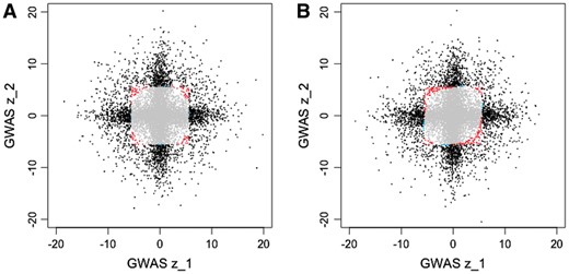
Rejection regions for MI GWAS and CONFIT. We ran MI GWAS and CONFIT on simulated GWAS summary statistics in two traits with simulation settings ${\lambda }_2\sim N(0,25)$ for (A) uncorrelated and (B) correlated studies. In each plot, the variants are color coded black if significant by both MI GWAS and CONFIT (i.e. MI GWAS P-value $\le 2.5\times {10}^{-8}$ and CONFIT P-value $\le 5\times {10}^{-8}$⁠), red if found significant by CONFIT but not MI GWAS, blue if found significant by MI GWAS and not CONFIT, and grey if not found significant by either method

In real datasets, it is possible that some traits will tend have larger or smaller effects than others. To see how CONFIT performs in this case, we also ran simulations where non-zero effects for one trait are drawn from ${\lambda }_{s1} N(0,4)$ and ${\lambda }_{s1} N(0,100)$⁠, and non-zero effects in the remaining traits are drawn ${\lambda }_s\sim N(0,25)$⁠. We found that CONFIT still increases power when an effect is present in more than one trait (Table 5).

Table 5.

Power simulation in three traits with differing effect size distributions between traits

	1 active trait	2 traits	3 traits
${\lambda }_{s1}\sim N(0,4)$
GWAS in t1	0.013	–	–
MI GWAS	0.182	0.3404	0.474
CONFIT	0.198	0.384	0.552
${\lambda }_{s1}\sim N(0,100)$
GWAS in t1	0.581	–	–
MI GWAS	0.366	0.605	0.768
CONFIT	0.347	0.627	0.832

The power of univariate GWAS in t₁ is in italics. Bolded values indicate multi-trait method with highest power for each simulation.

Notes: In the first trait t₁, we draw true effect size ${\lambda }_{s1}\sim N(0,4)$ or λ_s ∼ N(0,100), and in the other two traits, we draw ${\lambda }_s\sim N(0,25)$⁠. The true probability for each alternate configuration is 0.5%. For GWAS in t₁, we only count simulated SNPs which truly have an effect in t₁.

3.3 CONFIT increases power in polygenic variants when applied to studies with overlapping cohorts

To model the scenario where each trait is measured in the same cohort, i.e. dependent studies, we simulate summary statistics with correlation Σ_Z between the z-scores across traits, using Σ_Z computed from the Northern Finland Birth Cohort (NFBC) low-density lipoprotein (LDL) and high-density lipoprotein (HDL) traits for simulations in two traits, and from LDL, HDL and triglycerides (TG) for simulations in three traits. We find that the Σ_Z estimated from the covariance between individual level phenotypes matches closely with Σ_Z estimated from summary statistics (results not shown). We then run CONFIT with the correction for overlapping individuals described in Section 2.7.

Again, we see that CONFIT achieves slightly less power than MI GWAS when the effect is present in one trait, and increased power when the effect is present in more than one trait (Tables 3 and 4). The rejection region for CONFIT is now shifted relative to the rejection region for CONFIT without the overlapping individuals assumption, as shown in Figure 1B.

3.4 CONFIT finds unique loci for metabolic traits in the NFBC

Next, we applied CONFIT to a real dataset, on metabolic traits from the NFBC dataset (Kang et al., 2010; Sabatti et al., 2009). This dataset contains 331 476 variants and 5326 individuals, with data collected in ten traits from each individual. These traits include a variety of metabolic traits. We selected the five traits with at least one SNP with a GWAS P-values less than ${10}^{-4}$ in two or more traits and ran CONFIT on their summary statistics. These traits were measurements for glucose (GLU), HDL, insulin level (INS), LDL and TG. Note that for MI GWAS with five traits, the significance threshold is $1\times {10}^{-8}$ for the minimum GWAS P-value out of the five traits.

We used pyLMM (https://github.com/nickFurlotte/pylmm) to obtain GWAS summary statistics on the full NFBC cohort for each trait under a linear mixed model (LMM) as in (Kang et al., 2010). Our GWAS results are consistent with those reported by a previous GWAS in the NFBC data also using LMMs (Kang et al., 2010). We report the univariate GWAS P-value in each trait as well as the CONFIT P-value in Table 6. For MI GWAS in five traits, the significance threshold is $1\times {10}^{-8}$⁠.

Table 6.

P-values of peak CONFIT SNPs in analysis of five metabolic traits in NFBC data

			Univariate GWAS
Chr	Position	rsID	GLU	HDL	INS	LDL	TG	CONFIT
CONFIT only
8	19875201	rs10096633	4.5E–01	3.0E–06	4.1E–01	9.3E–01	1.9E–08	8.0E–10
16	66570972	rs255049	8.4E–01	1.7E–08	7.3E–01	1.7E–01	1.9E–01	2.0E–08
MI GWAS only
19	11056030	rs11668477	8.3E–01	1.8E–02	1.4E–02	3.5E–09	1.7E–02	6.4E–08
Found by both CONFIT and MI GWAS
1	109620053	rs646776	8.8E–01	1.2E–01	1.0E–01	3.0E–15	7.6E–01	<2.0E–10
2	21047434	rs6728178	1.6E–01	6.7E–07	8.9E–01	4.8E–08	1.8E–07	<2.0E–10
2	27584444	rs1260326	2.4E–01	2.6E–01	3.2E–01	2.1E–01	1.9E–10	2.0E–10
2	169471394	rs560887	6.9E–13	8.8E–01	9.9E–01	3.8E–01	6.2E–01	<2.0E–10
7	44177862	rs2971671	4.4E–09	9.0E–01	2.4E–01	5.9E–01	5.4E–01	8.6E–09
11	92308474	rs3847554	2.4E–10	3.5E–01	1.3E–02	6.2E–01	5.9E–01	8.0E–10
15	56470658	rs1532085	2.3E–01	7.2E–12	5.1E–01	5.6E–01	8.8E–02	<2.0E–10
16	55550825	rs3764261	4.4E–01	1.0E–32	7.5E–01	2.8E–01	1.2E–01	<2.0E–10

Notes: Table contains loci found significant by CONFIT or MI GWAS. The traits used in the analysis are glucose (GLU), HDL, insulin (INS), LDL and triglyceride (TG) levels.

Table 7.

P-values of peak CONFIT SNPs in analysis of four metabolic traits in NFBC dataset

			Univariate GWAS
Chr	Position	rsID	CRP	HDL	LDL	TG	CONFIT
CONFIT only
8	19875201	rs10096633	3.9E–01	3.0E–06	9.3E–01	1.9E–08	4.0E–09
16	66570972	rs255049	7.8E–01	1.7E–08	1.7E–01	1.9E–01	4.2E–08
Found by both CONFIT and MI GWAS
1	109620053	rs646776	1.4E–01	1.2E–01	3.0E–15	7.6E–01	<2.0E–10
1	157908973	rs1811472	1.2E–15	4.8E–02	6.1E–01	8.7E–01	<2.0E–10
2	21047434	rs6728178	5.3E–02	6.7E–07	4.8E–08	1.8E–07	<2.0E–10
2	27584444	rs1260326	5.1E–02	2.6E–01	2.1E–01	1.9E–10	2.4E–09
12	119873345	rs2650000	2.2E–12	2.8E–01	6.8E–01	6.0E–01	<2.0E–10
15	56470658	rs1532085	7.1E–01	7.2E–12	5.6E–01	8.8E–02	<2.0E–10
16	55550825	rs3764261	3.2E–01	1.0E–32	2.8E–01	1.2E–01	<2.0E–10
19	11056030	rs11668477	8.7E–01	1.8E–02	3.5E–09	1.7E–02	3.4E–08

Notes: Table contains peak CONFIT SNPs for loci found significant by CONFIT or MI GWAS. Italics indicates the only locus found significant by (Furlotte and Eskin, 2015) in their joint analysis of all four traits.

Table 8.

P-values of peak SNPs in analysis of four metabolic traits in UKKB dataset

		Univariate GWAS
Chr	Position	rsID	High cholesterol	Cholesterol medication	Insulin medication	Elevated blood GLU	CONFIT
CONFIT only
3	135925191	rs1154988	5.2E–08	9.8E–07	7.2E–01	2.3E–01	5.6E–09
7	73020301	rs799157	3.2E–08	3.1E–05	5.4E–01	7.3E–01	3.9E–08
7	150690176	rs3918226	3.0E–08	3.0E–07	3.9E–01	1.9E–01	1.0E–09
10	94772638	rs10748588	2.3E–07	1.5E–06	8.7E–01	3.1E–01	3.0E–08
11	126225876	rs112771035	5.9E–07	4.2E–06	3.6E–02	8.0E–01	4.8E–08
20	17844492	rs2618567	1.6E–08	6.0E–07	3.9E–01	2.4E–01	1.0E–09

Notes: Table contains peak SNPs found significant by CONFIT (CONFIT P-value $\le$ 5E–08) only. SNPs found significant by MI GWAS only are shown in the Supplementary Material.

CONFIT finds two unique loci in the NFBC data compared to MI GWAS. One of these loci (Chr 16, peak SNP rs255049) is significant for HDL under a univariate GWAS threshold, and the other loci (Chr 8, peak SNP rs10096633) has been associated with TG in a larger study from 2010 (Kamatani et al., 2010). CONFIT missed one loci found by MI GWAS only which is GWAS significant for TG only, also shown.

3.5 CONFIT outperforms a multi-variate linear regression model when applied to multiple traits

Next, we compared the performance of CONFIT against another multi-trait analysis method. Previously, Furlotte et al. applied multivate regression with a LMM (implemented in their software mvLMM) to the NFBC dataset using four traits: C-reactive protein (CRP), HDL, LDL and TG (Furlotte and Eskin, 2015). When running mvLMM to CRP, HDL, LDL and TG simultaneously, Furlotte et al. found only one significant locus, which contains SNPs rs1811472, rs2794520, rs2592887 and rs12093699.

We applied CONFIT to the NFBC dataset in these same four traits, again using GWAS summary statistics generated by pyLMM. Results are shown in Table 7. CONFIT in fact finds this locus, as well as nine other loci which were all reported in the univariate LMM analysis performed by (Kang et al., 2010). CONFIT discovers the same loci in these four traits as in the analysis on GLU, HDL, INS, LDL and TG, with the exception of a GLU-specific locus. It also finds a locus (Chr 19, rs11668477) that it missed in the five trait analysis. Although CONFIT can discover SNPs with effects present in only a subset of traits in the analysis, the specific traits chosen will affect its performance.

3.6 CONFIT finds unique loci in the UKKB dataset

We also applied CONFIT to UKKB summary statistics publicly released by Neale lab. We selected four traits related to the metabolic traits we used in the NFBC data. These are: self-reported high cholesterol (phenotype code 20002_1473), use of cholesterol lowering medication (phenotype code 6177_1), use of insulin medication (phenotype code 6177_3) and diagnosis of elevated blood glucose level (phenotype code R73, ICD10 R73). CONFIT finds 6 unique loci (Table 8), MI GWAS finds 44 unique loci (shown in Supplementary Material) and 304 loci are found by both methods (not shown). The loci found by CONFIT are all close to GWAS significance in both the self-reported high cholesterol and use of cholesterol medication phenotypes, whereas the loci it fails to discover are mostly borderline GWAS significant in a single trait (Supplementary Table S1).

4 Discussion

Here, we present CONFIT, a method for detecting associated variants from independent GWAS in multiple traits using summary statistics. We demonstrate our method in simulated data on two and three traits, and on real data up to four traits, though this framework may be applied to larger numbers of traits. CONFIT controls the false positive rate and increases power relative to MI GWAS when the variant is active in multiple traits in the analysis. When the variant is only active in one trait, CONFIT is less powerful than MI GWAS, which is the standard method for analyzing independent traits, so CONFIT does not discover exactly the same SNPs as GWAS. We discover unique loci when applying CONFIT to summary statistics from the NFBC and UKKB datasets.

A related problem exists in the field of eQTL studies, which often collect gene expression data from individuals in multiple tissues. In this case, the phenotypes are a given gene’s expression levels in each tissue, and the problem is to find variants associated with the gene’s expression in at least one tissue. Several approaches have successfully increased power in these multi-tissue eQTL datasets. Examples include MetaTissue (Sul et al., 2013), RECOV (Duong et al., 2017) and eQTL-bma (Flutre et al., 2013). MetaTissue uses RE meta-analysis to combine data from different tissues. RECOV explicitly models correlation between studies using a covariance matrix. eQTL-bma uses configurations to allow heterogeneity and performs Bayesian model averaging using each potential configuration as a model. We note the similarity of our test statistic to that of eQTL-bma, which was developed by Flutre et al. specifically for multi-tissue eQTL context (Flutre et al., 2013). A variant is an eQTL if it is associated with the expression of any gene in any tissue, which is quite likely when there are large number of tissues. For this reason, methods developed for multi-tissue eQTL studies differ from those for traditional GWAS in that eQTL studies typically do not assume a sparse model. In contrast, the majority of variants are believed to have no effect on the majority of disease traits. Hence it is not obvious whether multi-phenotype analysis methods for eQTL studies are also applicable to GWAS. Our results suggest they may be applicable.

The CONFIT framework is general and there are many options for setting the priors on each configuration. Here, we used a relatively simple method to estimate the priors by counting the number of SNPs with GWAS summary statistics that match each configuration. One alternative is to formulate this as an optimization problem and select priors that explicitly maximize power, with some form of regularization to avoid overfitting. Another possibility is to use external information about the variants to set the prior. This has been done previously in eQTL data, where variants in regulatory regions receive a stronger prior for association (Duong et al., 2016).

The count-based prior used here has the disadvantage of not scaling well as the number of traits grows, since as the number of possible configurations grows exponentially, the probability of observing any particular configuration decreases sharply. From a methods viewpoint, count-based methods for setting the prior on each configuration become less and less useful with larger numbers of traits, as the probability of observing any particular configuration amongst the GWAS statistics decreases with the number of traits. From a computational viewpoint, the runtime of CONFIT grows exponentially. For these reasons, we do not recommend running CONFIT on more than 10 traits. If the user has a large set of candidate traits, they may narrow down which traits to include in the analysis by choosing sets of traits with overlapping GWAS significant SNPs. One may use the Jacquard index to measure overlap between traits while also accounting for the fact where one trait may simply have more significant SNPs than other traits.

It is common for GWAS datasets to share individuals between studies. For example, a study may collect both LDL and triglyceride levels from each individual, or controls may be shared across multiple case-control studies. CONFIT handles the cases where the studies use the same cohort by approximating the correlation between traits due to sharing of individuals as proportional to correlation between traits or association statistics. This assumes the effect and residuals are approximately independent, and that any individual SNP or LD block has small effect on the phenotype. In this paper, we assume heritability of 50% when estimating this correlation, but a more sophisticated approach would be to use trait-specific heritability estimates. There are also many other methods to address the issue of overlapping individuals. For example, MetaTissue uses LMMs to model effects in multiple studies with shared individuals (Sul et al., 2013). Although their method was designed for multi-tissue eQTL studies, a similar LMM approach could be applied to combine GWAS. This approach has the advantage of estimating the proportion of the phenotype that can be attributed to sharing of individuals, and applies even if there is only partial overlap between studies. However, it requires individual level data and is relatively computationally expensive.

Several methods for analyzing multiple traits require individual level genotype and phenotype data, such as multi-variate regression. Several methods, such as GEMMA-mvLMM, mvLMM and GAMMA, extend this to use LMMs, which allow for correction of population structure and other covariates (Furlotte and Eskin, 2015; Joo et al., 2016; Zhou and Stephens, 2014). As with traditional meta-analysis, multi-variate regression is not suitable for combining data on arbitary traits and may achieve sub-optimal power for detecting variants that only affect one of the traits tested, or in the case where the variant only affects one trait, which indirectly affects another (Stephens, 2013). Such methods are typically applied to sets of traits that are already believed to share an underlying genetic basis (Furlotte and Eskin, 2015). Thus there is a need for flexible approaches to association testing when the traits only partially share a genetic basis and the study cohorts are not independent between traits.

Funding

L.G. and E.E. was supported by National Science Foundation grants 0513612, 0731455, 0729049, 0916676, 1065276, 1302448, 1320589 and 1331176 and National Institutes of Health grants K25-HL080079, U01-DA024417, P01-HL30568, P01-HL28481, R01-GM083198, R01-ES021801, R01-MH101782 and R01-ES022282.

Conflict of Interest: none declared.