PrimAlign: PageRank-inspired Markovian alignment for large biological networks

Abstract

Motivation

Cross-species analysis of large-scale protein–protein interaction (PPI) networks has played a significant role in understanding the principles deriving evolution of cellular organizations and functions. Recently, network alignment algorithms have been proposed to predict conserved interactions and functions of proteins. These approaches are based on the notion that orthologous proteins across species are sequentially similar and that topology of PPIs between orthologs is often conserved. However, high accuracy and scalability of network alignment are still a challenge.

Results

We propose a novel pairwise global network alignment algorithm, called PrimAlign, which is modeled as a Markov chain and iteratively transited until convergence. The proposed algorithm also incorporates the principles of PageRank. This approach is evaluated on tasks with human, yeast and fruit fly PPI networks. The experimental results demonstrate that PrimAlign outperforms several prevalent methods with statistically significant differences in multiple evaluation measures. PrimAlign, which is multi-platform, achieves superior performance in runtime with its linear asymptotic time complexity. Further evaluation is done with synthetic networks and results suggest that popular topological measures do not reflect real precision of alignments.

Availability and implementation

The source code is available at http://web.ecs.baylor.edu/faculty/cho/PrimAlign.

Supplementary information

Supplementary data are available at Bioinformatics online.

1 Background

Recent high-throughput techniques have been exploring protein functions and interactions with other proteins. Apart from experimental studies, computational analyses over existing data are also performed, as they are considerably faster, less expensive and their predictions of interactions and functions can substantially expedite new discoveries. These works have made genome-wide protein–protein interaction (PPI) data publicly available, collectively referred to as Interactome. (Koh et al., 2012; Rolland et al., 2014).

From the standpoint of comparative Interactomics, cross-species comparison of the link patterns in PPI networks have played a significant role in this field, since it increases our understanding of principles deriving evolution of cellular organizations and functions (Sharan et al., 2005). This type of computational analysis is called network alignment. It is based on a formal view of PPI networks as graphs, where proteins are represented as nodes and their interactions as edges. PPI networks of two species are aligned together in the sense that proteins with the identical function are mapped to each other. This is possible, since many genes and proteins are conserved in similar forms across different species; they are called orthologs. Based on the alignment results, further topological and functional analyses can be performed. Interactions in one network can point towards possible interactions in the other network. Similarly, functions of a protein in one network can predict functions of another protein aligned to it from the other network if they are true orthologs.

Various network alignment algorithms have been proposed over the last decade so as to predict conserved interactions and functions of proteins. Network alignment algorithms are divided into two groups: global network alignment and local network alignment. The former deals with aligning entire networks and aims at finding the maximal set of mapped node pairs. On the other hand, the latter searches for a set of sub-structures that represent conserved functional components. Sometimes, this distinction is being simplified to many-to-many mappings for local aligners and one-to-one mappings with pairing all nodes from the smaller network for global aligners. We follow the former distinction based on production of conserved clusters, as we have observed that some global aligners produce many-to-many mappings and do not connect all proteins from the smaller network. Earlier studies handled local alignment for aligning small networks whereas most recent studies have proposed global alignment algorithms for large-scale PPI networks.

One of the earliest local alignment tools was PathBLAST (Kelley et al., 2004) which discovers conserved pathways by pairing interactions between orthologous proteins. It takes a query pathway and aligns it to a PPI network, outputting all matching paths from the network which achieve a certain threshold score. The score of each path is based on the BLAST (Altschul et al., 1990) e-value of each aligned protein pair, as well as the ‘probability of a real interaction’ between proteins along the path, defined as the number of studies which confirm each interaction. NetworkBLAST (Kalaev et al., 2008), as an upgraded version of PathBLAST, allows for performing alignment between multiple networks to identify two types of shared sub-graphs: linear paths of interacting proteins (i.e. signaling pathways) and clusters of densely interacting proteins (i.e. protein complexes). It searches for highly similar sub-networks and extends them in a greedy manner. MaWISh (Koyuturk et al., 2006) is a graph-theoretic optimization model to solve the maximum weight induced sub-graph problem. It iteratively searches for a match, mismatch and duplication of interactions between two PPI networks to discover highly conserved groups of interactions, inspired by the duplication and divergence model for PPI network evolution. Recently, PINALOG (Phan and Sternberg, 2012), AlignNemo (Ciriello et al., 2012) and AlignMCL (Mina and Guzzi, 2014) have been introduced as local aligners.

As for global alignment algorithms, IsoRank (Singh et al., 2008) is the first algorithm that applies the concept of PageRank to network alignment. It computes a score for each node based on the principle that neighboring nodes of the nodes aligned to each other should also be aligned to each other in the other network. It computes a steady-state distribution combined with a personalized PageRank vector. The upgraded version, IsoRankN (Liao et al., 2009), uses a spectral clustering to efficiently produce a multiple alignment, leaving the previous version obsolete. SMETANA (Sahraeian and Yoon, 2013) and CUFID (Jeong et al., 2016) perform a Markov random walk in the joined network to compute a steady-state distribution. Additional probabilistic consistency transformations are executed on the results. In addition, CUFID calculates steady-state flow through the edges and applies a bipartite matching to obtain one-to-one alignment. In contrast, SMETANA allows for many-to-many alignment where one protein from one network can be aligned to multiple proteins from the other network.

Most of the global alignment algorithms maximize alignment score which is computed by a combination of sequence similarity and topological similarity for protein pairs from two (or more) PPI networks. Recently proposed global aligners include MI-GRAAL (Kuchaiev and Pržulj, 2011), L-GRAAL (Malod-Dognin and Pržulj, 2015), SPINAL (Aladağ and Erten, 2013), NETAL (Neyshabur et al., 2013), NetCoffee (Hu et al., 2014), HubAlign (Hashemifar and Xu, 2014), MAGNA (Saraph and Milenković, 2014), MAGNA++ (Vijayan et al., 2015), WAVE (Sun et al., 2015) and SANA (Mamano and Hayes, 2017).

In this paper, we propose a new global network alignment method called PrimAlign––PageRank-Inspired Markovian Alignment. This algorithm is built upon the idea of modeling the networks as a Markov chain that is iteratively transited until convergence, combined with the basic principles of the original PageRank algorithm and sparse computations. The multi-platform source code in C# is provided. The method is compared with several previous network alignment algorithms introduced above while performing pairwise alignment of human, yeast and fruit fly networks. The proposed method performs superiorly to the other algorithms with respect to the alignment quality as well as computation time. Additional evaluation is performed with 30 synthetic networks from the popular set, NAPAbench (Sahraeian and Yoon, 2012).

2 Materials and methods

2.1 Markov chains

In computational modeling, Markov chains are well-established models describing discrete sequences of stochastic processes, in which the following state depends only on the current state. Markov chains consist of possible states, in which the system under consideration can be found and probabilities of transition from each state to each other state when performing a step in the process sequence. As the model is stochastic, the overall state of the system at each step is described as a probability distribution over all possible states, expressing the probability of the system being currently in each particular state.

Since the model topology is fixed and transition probabilities are constant, a Markov chain can be defined by a constant transition matrix $T$⁠, in which the value at row $i$ and column $j$ represents the probability of transition from state $S_i$ to state $S_j$ at step $t$ when being in state $S_i$⁠:

$$T\left[i.\hspace{0.17em}j\right]=P\left(S_j^{\left(t+1\right)}||S_i^{\left(t\right)}\right)$$

The state distribution at step $t$ can be represented as a vector $p$⁠, where the value at index $i$ represents the probability of being in state $S_i$⁠:

$$p^{\left(t\right)}\left[i\right]=P\left(S_i^{\left(t\right)}\right)$$

This formula allows for straightforward computation of subsequent states:

$$p^{(t+1)}=p^{\left(t\right)}T$$

$$p^{(t+2)}=p^{(t+1)}T=p^{\left(t\right)}TT$$

In Markov chain models, the usual task is to analyze the long-term state distribution $\pi$⁠, which can be stationary:

$$\pi =\underset{t\to \mathrm{ \infty }}{\lim }{p}^{\left(t\right)}$$

$$\pi =\pi T$$

However, reaching the stationary distribution is not guaranteed unless the chain is ergodic, which requires the transition matrix to be primitive.

2.2 PageRank

The original PageRank algorithm (Langville and Meyer, 2006) is based on representation of web pages as a Markov chain. The pages themselves are states while the links connecting them are possible transitions with non-zero probabilities simulating random browsing. The task is to find the stationary distribution. Due to the model topology, web pages with multiple incoming links or with links coming from important pages will be also important, i.e. they achieve a relatively high probability in the stationary distribution. To overcome the convergence problems, two modifications are incorporated into the transition matrix: First, states with no transition (pages with no links) are assigned with transitions to all other states with uniform probability. This step turns the transition matrix into a true right stochastic matrix. Second, a damping factor $\mathrm{\alpha }$ is introduced to simulate a chance of sudden ‘teleportation’ to a random state, which can occur with the probability of (1–$\mathrm{\alpha }$⁠). This change converts the transition matrix into a primitive stochastic matrix and its convergence during the iterative traversal is guaranteed. The modifications are not performed over the transition matrix directly, but rather the transition step is adjusted to:

$$p^{\mathrm{t}\mathrm{e}\mathrm{m}\mathrm{p}}=\mathrm{\alpha }\mathrm{ }{p}^{\left(t\right)}\left(T+\frac{q\mathrm{ }e}{n}\right)+\left(1-\mathrm{\alpha }\right)\frac{e^{T}e}{n}$$

$$p^{(t+1)}=\frac{p^{\mathrm{t}\mathrm{e}\mathrm{m}\mathrm{p}}}{{‖\Vert p^{\mathrm{t}\mathrm{e}\mathrm{m}\mathrm{p}}‖\Vert }_1}$$

where: $\mathrm{\alpha }=\hspace{0.5em}$ damping factor $q=\hspace{0.5em}$ column vector (length $n$⁠), for each row of $T$⁠: 1 if the row is all-zero, 0 otherwise. $e=\hspace{0.5em}$ row vector of 1 s (length $n$⁠). $T=\hspace{0.5em}$ transition matrix (size $n\hspace{0.5em}\times \hspace{0.5em}n$⁠). $n=\hspace{0.5em}$ number of states. $p^{\mathit{(t)}}=\hspace{0.5em}$ state probability distribution vector at step $t$ (length $n$⁠).

While $qen$ represents the first modification, (⁠$1-\mathrm{\alpha })e^{T}e/n$ introduces the teleportation effect. The temporary variable $p^{\mathrm{t}\mathrm{e}\mathrm{m}\mathrm{p}}$ is normalized by its L1-norm, so that the result is a valid probability distribution vector.

The smaller the damping factor is and the larger the probability of the random teleportation is, the more affected the results are and the probability distribution is smoothened although convergence is faster. Nevertheless, every damping factors smaller than 1 guarantee the convergence.

2.3 PrimAlign

Our new method searches for stationary-distributed transition probabilities between two joined PPI networks forming a Markov chain with PageRank-inspired modifications. While the idea of Markov random walk was previously used in CUFID and a personalized PageRank vector was used in IsoRank, the proposed PrimAlign algorithm is built upon both the Markovian representation and PageRank modifications with sparse computations, nicely integrating similarity weights with the network topology and guaranteeing the convergence and achieving linear time complexity (linear with respect to the number of edges on input), which is the theoretical minimum for this task. Supplementary Figure S1 shows individual steps in the data flow of PrimAlign.

Input: Three files are expected on input. The first two represent PPI networks which are to be aligned. Any edges can be weighted to specify the interaction confidence. The third file lists sequence similarities of inter-network protein pairs, all of which are treated as candidate orthologs. The recommended sequence similarity score is either BLAST bit-score or -log of BLAST e-value. The fourth parameter is the output file path. Optionally, a threshold for selecting orthologs can be provided, otherwise the program uses a default threshold (0.75). The exact specification of input and all file formats are detailed in Supplementary Text S1.

Edge reweighting: The sequence similarity scores are cubed. Thanks to the normalization in the next phase, this exponentiation amplifies the ratios between individual scores (large scores become even larger and small scores become even smaller), while they still sum up to 1. Different exponents were explored, and the effect is visible as long as any exponentiation occurs, so the exact exponent could have been set differently with a little change in results (Supplementary Fig. S2). The motivation behind this step is the assumption that differences in sequence similarity are more relevant than differences in network topology and protein interaction weights, so the differences in sequence similarity are amplified.

Building transition matrix: The transition matrix is first built as a symmetric square matrix with one row and one column for each protein detected across the input files. The number at row r and column c represents a similarity weight between r-th and c-th protein or zero if the protein pair is not defined in any input file. This weight is either PPI similarity if the proteins come from the same network (or 1, respectively, if PPI weights are not specified in the input file), or reweighted sequence similarity if the proteins come from different networks. Then, the matrix is normalized to form a valid transition matrix by scaling each row to sum up to 1. If a protein can transit both within its network and into the other network, its weights are scaled so that the total probability of transiting within its network is the same as the total probability of transiting into the other network. Alternatively put, we can imagine the whole matrix as a composition of four partial transition matrices depending on whether the source and destination of the transition is network $A$ or $B$⁠:

$$T=\left[\begin{array}{cc}{T}_{A\to A}& T_{A\to B}\\ T_{B\to A}& T_{B\to B}\end{array}\right]$$

where: $T_{A\to A},T_{B\to B}=\hspace{0.5em}$ partial matrices with same-network transitions built from PPI network weights. $T_{A\to B},T_{B\to A}=\hspace{0.5em}$ partial matrices with inter-network transitions built from sequence similarity weights.

In this view, the normalization can be done as row normalization of the partial matrices with subsequent row normalization of the whole matrix.

PageRank-inspired stationary distribution computation: Starting with a uniformly-distributed probability vector over the proteins, the transition matrix is repeatedly traversed and the probability vector is updated. The iteration ends when a stationary distribution is reached (1e–5 in L2-norm change of the vector π) or after a maximum number of iterations (200, but in our experiments it typically converges within 20 iterations). The algorithm is inspired with PageRank by including its two principles mentioned earlier: Proteins with no transitions (which could occur when a protein is listed on input, but all its weights and scores are 0) simulates transitions to all other proteins with uniform probability, and the damping factor α is included to simulate random ‘teleportation’ from each protein. This change converts the transition matrix into a primitive stochastic matrix and its convergence during the iterative traversal is guaranteed. α was set to 0.85 as in the original PageRank algorithm (Langville and Meyer, 2006). This parameter seems to be robust as well (Supplementary Fig. S2).

As the number of proteins in both species can be relatively large, resulting in matrix M with around 1 000 000 000 elements, and because of repeated vector-matrix multiplications, it is crucial to represent the matrices as sparse objects. Otherwise, the computation load would be unfeasible for computation with real-world PPI networks in a genomic scale. The formula stated above is in a form allowing simple reading of the incorporated PageRank modifications, but operates with full non-sparse matrices and the performance would be degraded greatly. Therefore, the real equation used is based on a form converted by regrouping the algebraic elements, so that the sparse computations may be preserved:

$$p^{\mathrm{t}\mathrm{e}\mathrm{m}\mathrm{p}}=\mathrm{\alpha }\mathrm{ }{p}^{\left(t\right)}T-\left(\mathrm{\alpha }\mathrm{ }{p}^{\left(t\right)}q+1-\mathrm{\alpha }\right)\frac{e}{n}$$

Inter-network traversal probabilities extraction: Traversal probability is computed for each inter-network protein pair (candidate ortholog) as the stationary probability for one protein multiplied by the probability of selecting its paired protein as a transition target out of other possible inter-network transitions (within-network transitions are of no interest now), and summed symmetrically with the probability computed in the same manner for the other protein in the pair. As the probabilities rather dissolve with the increasing number of proteins, the final score results from normalization of the traversal probabilities by multiplication with the number of unique proteins. This ensures that the values are comparable across alignments of networks of varied sizes. Formally, for $a$-th protein from network $A$ and $b$-th protein from network $B$⁠:

$$\mathrm{s}\mathrm{c}\mathrm{o}\mathrm{r}\mathrm{e}\left(a,b\right)=\left(\pi \left[a\right]\frac{T_{A\to B}\left[a,b\right]}{\Vert {‖T_{A\to B}\left[a,\mathrm{ }1:n_B\right]‖\Vert }_1} +\pi \left[n_A+b\right]\frac{T_{B\to A}\left[b,a\right]}{\Vert {‖T_{B\to A}\left[b,\mathrm{ }1:n_A\right]‖\Vert }_1}\right)n$$

where: $n,n_B=\hspace{0.5em}$number of proteins in network $A,B$⁠.

Thresholding: The cut-off threshold to apply to the final score to select high-quality ortholog candidates is 0.75 by default and can be user-defined on input. We recommend using a number between 0.5 [more permissive, more false positives (FPs)—likely to select proteins that are not real orthologs] and 1 [more strict, more false negatives (FNs)—likely to miss some real orthologs]. The effect of these threshold values is shown in Supplementary Figure S3. Setting the threshold to 0 outputs all ortholog candidates.

Output: Ortholog candidates with the scores greater or equal to the threshold are written to a file specified on program input together with their scores in a tab-delimited format (Supplementary Text S1).

3 Experiment design

3.1 Data acquisition

In this study, the PPI networks of human (Homo sapiens), yeast (Saccharomyces cerevisiae) and fruit fly (Drosophila melanogaster) were selected, as they are well-explored and of a reasonable size. All the networks were acquired from BioGRID (Chatr-aryamontri et al., 2017) and filtered for physical interactions. The interacting proteins were paired with genes that they are produced by, and maintained and treated as gene-to-gene interactions. This approach helps with connecting information from multiple databases together.

Semantic information was provided through ontology annotations. The annotation files were downloaded from GO (The Gene Ontology Consortium, 2015) containing over 400 000 annotations with GO terms for human, and over 100 000 GO annotations for yeast. Only pairs, in which the genes have at least one GO annotation, were considered. GO itself was used in the basic version to guarantee safe propagation of annotations within the ontology hierarchy and all types of GO relationships were treated equally for the purpose of creating a parent-child hierarchy and subsequent annotation propagation. Annotations marked as IEA (Inferred from Electronic Annotation) were excluded.

The genes were further annotated with KEGG Orthology (KO) functional annotations (Kanehisa et al., 2017), which describe molecular functions of genes and proteins and can be used for orthology matching. Furthermore, two lists of high-confident orthologous genes were obtained. The first was exported through ENSEMBL BioMart (Kinsella et al., 2011) and the other was downloaded from InParanoid (Sonnhammer and Östlund, 2015). While all of these three sources partially rely on sequence similarity when finding matching pairs, each method approaches the task differently. While InParanoid employs a pairwise BLAST-based approach, ENSEMBL uses a phylogeny-based method and KO functional annotations undergo a comprehensive check against pathways of multiple species in KEGG database and are partially manually reviewed. We assume these sets contain true orthologs even though they may be highly incomplete (there may be many orthologs undetected by these methods).

To map individual datasets together, various types of identifiers were connected via UniProt mapping service (The UniProt Consortium, 2017). These include: UniProt KB protein IDs, UniProt KB gene IDs, gene names and their synonyms, BioGRID protein IDs, Saccharomyces Genome Database gene IDs, ENSEMBL gene IDs. Synonyms were considered as long as they did not collide with other names.

Overall, the transformations and filtering resulted in the networks of almost 270 000 interactions of 16 000 unique genes for human, almost 90 000 interactions of 6000 unique genes for yeast and more than 41 000 interactions of 14 000 unique genes for fruit fly. KO annotations were available for over 12 000 human genes, 3000 yeast genes and almost 6000 fruitfly genes. ENSEMBL and InParanoid lists contain almost 6000 and 2000 human-yeast orthologs, 13 500 and 4500 human-fruit fly orthologs and 5000 and 2000 yeast-fruit fly orthologs.

3.2 Alignment task

All three pairwise combinations of the three networks were aligned with PrimAlign as well as the following algorithms for comparison: AlignMCL, AlignNemo, CUFID, HubAlign, IsoRankN, MAGNA++, MI-GRAAL, NETAL, NetCoffee, NetworkBLAST, PINALOG, SANA, SMETANA and WAVE. Thus, we do not avoid comparison with both global and local aligners, since both categories attempt to discover correct functional orthologs at first, regardless of whether they additionally group them into conserved clusters or not and whether they assume one-to-one mappings or not. We compare them directly at the same size of output to avoid a possible bias caused by isolation of high confidence pairs comparing to more complete mappings as explained in Section 3.3.

On input, the algorithms accept a network file for each species with a list of interacting pairs, either unweighted or weighted according to the interaction strength. Another input is sequence similarity of pairs between the networks as produced by BLAST analysis, or within each network as well for some algorithms. We computed the PPI weights in two forms: (i) as semantic similarity scores, called sim_GIC (Pesquita et al., 2008), and (ii) all set to 1, making them effectively unweighted. This enables us assessing the effect of weighting using semantic similarity.

Sequence similarity on input is an essential part of biological network alignment. Without it, an algorithm could just optimize the topological similarity, which is prone to overfitting and missing the true functional matches, especially in incomplete networks. The input BLAST information is either BLAST bit-score or BLAST e-value. The main difference between them is that the e-value is adjusted according to lengths of protein sequences, so the e-value and the bit-score are not directly convertible without knowing the protein lengths and the total size of the BLAST library. Nevertheless, the algorithms accept a form of both except NetworkBLAST which is strict in demanding e-values. Therefore, the e-value measure was used for all the algorithms. The datasets bundled with NetCoffee have been processed for this purpose. As a result, the BLAST files contain the scores of over 60 000 human-yeast pairs, 40 000 human-fruit fly pairs, 9000 yeast-fruit fly pairs, 200 000 human-human pairs, 30 000 yeast-yeast pairs and 8000 fruit fly-fruit fly pairs.

IsoRankN is applicable with weighted networks, but in fact, its authors do not recommend inserting weights due to insufficient testing of the algorithm for weighted data. Therefore, only unweighted networks have been used for IsoRankN. Binaries available for NetCoffee are not up-to-date and are marked as obsolete although new source files are available. Therefore, the latest code from their Git repository was compiled and used for comparison. It was discovered that CUFID and SMETANA share a bug of rewriting network weights: Although both algorithms read and store the weight values, they are later ignored and replaced by 1s. As a result, the outputs were identical when using either of the weighting methods. Be it a bug or a feature, we have fixed the code to process the weights.

Additionally, we have restricted PrimAlign in two forms to process either only sequence similarities without any network files on input (PrimAlign-Seq), or only topology of unweighted networks without sequence similarities (PrimAlign-Topo). These versions serve for comparison of contribution of topology information and sequence similarities to the final power of PrimAlign.

All the algorithms and their inputs are summarized in Table 1. The parameters were selected according to recommendations from provided manuals with respect to the size of the tasks or default values were used. Processing of sequence similarities as well as multi-threading was always enabled (if applicable). The log transformations of e-values equal to 0 have been substituted by log of the smallest positive value that a number of double precision could represent.

Table 1.

Summary of algorithms for comparison

Algorithm	BLAST data	Algorithm parameters	Weights	One-to-one	Enforced coverage	Type
AlignMCL	-log2 (e-value) inter-network		Yes	No	No	Local
AlignNemo	e-values inter-network		Yes	No	No	Local
CUFID	-log2 (e-value) inter-network		Yes	Yes	No	Global
HubAlign	-log2 (e-value) inter-network		No	Yes	Yes	Global
IsoRankN	-log2 (e-value) intra & inter-network	-K 10 –thresh 1e–5 –alpha 0.7 –maxveclen 2000000	No	No	No	Global
MAGNA++	-log2 (e-value) inter-network	-p 15000 -n 2000 -a 0.5 -t 4 -m S3	No	Yes	Yes	Global
MI-GRAAL	-log2 (e-value) inter-network	-p 19	No	Yes	Yes	Global
NETAL	-log2 (e-value) intra & inter-network	-b 0.5 -c 0.5	No	Yes	No	Global
NetCoffee	e-values intra & inter-network		No	Yes	No	Global
NetworkBLAST	e-values inter-network	beta 0.9; blast_th 1e–30; true_factor0 0.5; true_factor1 0.5	Yes	No	No	Local
PINALOG	-log2 (e-value) inter-network		No	Yes	No	Local
SANA	-log2 (e-value) inter-network	-s3 0.5 -sequence 0.5	No	Yes	Yes	Global
SMETANA	-log2 (e-value) inter-network		Yes	No	No	Global
WAVE	-log2 (e-value) inter-network		No	Yes	Yes	Global
PrimAlign-Seq	e-values inter-network		No	No	No	Global
PrimAlign-Topo	unweighted inter-network		No	No	No	Global
PrimAlign	-log2 (e-value) inter-network		Yes	No	No	Global

Note: Enforced coverage means that all proteins from the smaller network need to be aligned.

Computation times of the algorithms were also compared. To guarantee a fair comparison, all algorithms were run on the same machine, with 8 GB RAM and quad-core 3 GHz CPU; either in Windows 10 environment (CUFID, SMETANA, PrimAlign) or Ubuntu Server 16.10 (others) and without active usage of the machine for other tasks (after reboot). Both environments enable multi-core processing. The time of start and end of runs was monitored programmatically and rounded to seconds.

3.3 Evaluation metrics

The output of each algorithm is a list of putative orthologous pairs. If an algorithm outputted a different structure, e.g. pairs in clusters of conserved regions, we always transformed the results into aligned pairs, the basic unit of alignment. Multiple measures were computed over the pairs to see basic statistics of alignments and to assess the alignment quality.

Four groups of evaluation measures are summarized and detailed in Table 2. Informative measures are included for overall statistics of the alignment: the size of the output (i.e. the number of aligned pairs), gene coverage (number of genes that are aligned), the number of conserved edges (an edge from one network that is aligned to an edge in the other network) and the size of the largest conserved connected component (LCCC). The first three measures are well-defined. LCCC represents the lower number of edges in the largest common connected sub-graph (LCCS) as defined in (Kuchaiev et al., 2010). To avoid any ambiguity, we define it as the number of edges in the largest connected component from one network consisting of conserved edges that map to a connected component in the other network (and then can be mapped back to itself), for which the network with the smaller projection of the component is selected (due to many-to-many mapping, the component in each network can have a different number of edges). LCCS can be characterized by both the number of edges and nodes. For simplicity, we chose only the former variant, preferentially because it reflects the density of LCCS and the number of conserved relationships. These informative measures are not meant for evaluation of the alignment quality. Note that here we included several topological measures that are sometimes used directly for evaluation. However, we consider such a usage pre-mature. Natural changes in topology (e.g. deletion), especially in the networks that are still incomplete, can result in functional conservation which is topologically sub-optimal, in which case topologically optimal alignment could have little biological meaning. Therefore, topological evaluation measures can be misleading.

Table 2.

Overview and classification of evaluation measures

	Abbr.	Measure	Calculation
Informative measures	AP	Aligned Pairs	# of aligned pairs
	Cov	Coverage	# of unique aligned genes
	CE	Conserved edges	# of edges from one network that are aligned to an edge in the other network
	LCCC	Largest conserved connected component	# of edges in the largest connected component assembled from conserved edges
Annotation-based measures	KO	KO functionally correct alignments	# of aligned pairs where both genes share KO functional annotation
	GO	GO semantically correct alignments	Sum of ratios of GO annotations shared by aligned pairs (i.e. sum of Jaccard indices)
Ground-truth-based measures	EN	Discovered ENSEMBL orthologs	# of ENSEMBL orthologs found among aligned pairs
	IP	Discovered InParanoid orthologs	# of InParanoid orthologs found among aligned pairs
Combined topological measures	CE-F	Conserved edges of functionally correct pairs	# of edges from one network that are aligned to an edge in the other network with both aligned gene pairs being functionally correct
	CE-O	Conserved edges of known orthologs	# of edges from one network that are aligned to an edge in the other network with both aligned gene pairs being among ENSEMBL or InParanoid orthologs
	LCCC-F	Largest conserved connected component from functionally correct pairs	# of edges in the largest connected component assembled from conserved edges between functionally correctly aligned pairs
	LCCC-O	Largest conserved connected component from known orthologs	# of edges in the largest connected component assembled from conserved edges between aligned pairs also present among ENSEMBL or InParanoid orthologs

The other three groups are computed to assess the alignment quality. In all quality measures, the higher value implies the better alignment. Annotation-based measures use either functional annotations from KO to indicate how many aligned pairs are aligned functionally correctly (share a KO annotation), or GO to evaluate how big the shared semantic context is (in terms of Jaccard indices of annotated GO terms). Ground-truth based measures consider the lists of orthologous genes from ENSEMBL and InParanoid and express how many of them were identified among the aligned pairs. Combined topological measures are derived from topological informative measures but combined with the previous two groups: Only either functionally correct aligned pairs (those sharing a KO annotation) or ground-truth correct aligned pairs (those among the lists of orthologs) are considered here. Combining topological measures with the other measures seems to be a more reasonable approach than using topological measures alone.

In order to evaluate alignments with various numbers of aligned pairs, annotation-based and ground-truth-based evaluation measures are complemented with their cost forms, saying how many aligned pairs on output are needed on average per one unit of the given evaluation measure. Formally for each measure X,

$$cX=\frac{\#\mathrm{ }\mathrm{a}\mathrm{l}\mathrm{i}\mathrm{g}\mathrm{n}\mathrm{e}\mathrm{d}\mathrm{ }\mathrm{p}\mathrm{a}\mathrm{i}\mathrm{r}\mathrm{s}}{X}$$

The cost measures have the opposite semantic than the other measures: The higher the cost value is, the lower the performance. However, these measures serve only as a hint for cross-algorithm comparison, as the scores are adjusted only in a linear manner with respect to the number of aligned pairs––and this assumption of linearity is not valid as shown in the Results Section. Instead, algorithms tend to produce more accurate pairs first and less accurate predictions with the growing output. This is not surprising (it is fully in the spirit of ROC curve), but it makes the comparison more difficult; e.g. accuracy of two algorithms with a distinct output size should not be directly compared.

Therefore, PrimAlign was additionally run to produce the same number of aligned pairs as the other algorithms for a fair individual comparison at the same size of output. To achieve this, we set the optional threshold parameter in PrimAlign to 0 to output all candidate orthologs and their scores and then we always selected the desired number of top pairs with the highest score, as if the threshold was set to produce the right number of pairs.

Statistical evaluation of the performance differences between Prim-Align and the other algorithms has been performed using two-proportion two-tailed z-test for measures, where each pair or edge can be marked as either positive or not (i.e. all evaluation measures except for GO) and using two-tailed Welch’s t-test for measures, where each edge contributes to a real value (only GO). P-value ≤ 0.05 was considered significant.

3.4 Synthetic networks

Next, we have performed another set of tests with 30 synthetic networks NAPAbench, each time aligning networks with 4000 and 3000 proteins. The networks are constructed by applying three different evolutionary models, which incorporate common biological events such as gene deletions, gene duplications, gene mutations and new functional specialization, followed by adjusting similarity scores. Although the models are based on certain assumptions, they have been shown to reflect multiple statistical properties of real evolution (Sahraeian and Yoon, 2012).

Comparing to real biological networks, synthetic networks have the advantage that the functional assignments are known, i.e. we know all true orthologs. Therefore, we can directly evaluate performance of the algorithms in terms of true positives (TP), FPs and FNs, consolidated as precision $\mathrm{T}\mathrm{P}$ and recall $\mathrm{T}\mathrm{P}$⁠. Thus, we do not have to rely on estimating the performance based on topology measures or incomplete sets of orthologs. However, we compute other measures designed for comparing local and global aligners (Meng et al., 2016), namely generalized symmetric sub-structure score (GS³) and node coverage combined with GS³ (NCV-GS³).

In this test, we compared PrimAlign with SANA and AlignMCL at their size of output as well as using the default threshold. SANA and AlignMCL were selected as superior global and local aligners, respectively, based on the results in the first part of our evaluation.

4 Results

4.1 Overview of alignment results

As an overview of the produced outputs, the informative measures and informative cost forms of the annotation-based and ground-truth-based measures are summarized in Table 3. These results are only descriptive and the highest or lowest values do not imply the best or worst performance although the cost measures serve as a hint for comparison.

Table 3.

Alignment overview with informative measures

Aligner	Weighted	AP	Cov	CE	LCCC	cKO	cGO	cEN	cIP
AlignMCL	No	7711	7064	19 528	7716	4.39	3.34	2.80	6.00
AlignMCL	Yes	7711	7064	19 528	7716	4.39	3.34	2.80	6.00
AlignNemo	No	4776	2826	9385	3936	4.37	3.24	3.09	6.46
AlignNemo	Yes	4081	2515	8127	3425	4.43	3.28	3.21	6.38
CUFID	No	5654	11 308	13 892	6664	4.54	4.34	4.03	5.30
CUFID	Yes	5250	10 500	14 744	7070	4.14	3.78	3.69	4.85
HubAlign	No	5926	11 852	50 016	24 978	5.19	4.36	4.50	5.99
IsoRankN	No	2964	5065	8711	3945	2.18	2.80	1.93	2.53
MAGNA++	No	5933	11 866	3388	1601	11.19	6.10	9.10	13.93
MI-GRAAL	No	NA	NA	NA	NA	NA	NA	NA	NA
NETAL	No	3100	6200	456	129	∞	7.74	3100	∞
NetCoffee	No	2310	4620	3742	1654	2.94	2.85	2.62	3.68
NetworkBLAST	No	7904	3185	12 552	5224	6.68	3.47	4.46	9.81
NetworkBLAST	Yes	4008	2195	10 404	4432	5.37	3.47	4.06	7.68
PINALOG	No	5317	10 634	32 792	16 285	4.19	4.01	3.76	4.70
PrimAlign	No	3801	4883	16 518	6971	2.31	2.86	1.71	3.07
PrimAlign	Yes	3752	4843	16 408	6934	2.29	2.86	1.70	3.04
SANA	No	5933	11 866	43 524	21 738	9.11	5.14	7.43	11.03
SMETANA	No	3487	5384	18 770	8981	2.83	2.97	2.31	3.46
SMETANA	Yes	3854	5718	14 417	6320	2.86	3.03	2.28	3.55
WAVE	No	5933	11 866	32 500	16 138	10.85	5.48	9.90	12.68

For human-yeast network alignment, the number of aligned pairs on output ranges between 2310 (NetCoffee) and 7904 (NetworkBLAST). Using the default threshold, PrimAlign produced 3801 pairs or 3752 pairs when using unweighted or weighted PPI networks, respectively. The highest coverage of proteins was achieved with MAGNA++, SANA, WAVE and HubAlign, as they enforce full coverage of the smaller network (HubAlign actually missed a few proteins lacking interaction). HubAlign also reached the highest number of conserved edges and LCCC.

The cost measures point towards inefficiencies in MAGNA++, SANA, WAVE, but also NetworkBLAST, which tend to produce more aligned pairs, seemingly less confident pairs. On the other hand, AlignMCL also produced a high number of aligned pairs, but its cost measures are relatively lower, suggesting it performs qualitatively better than them. Aligners with smaller output achieved lower costs except for NETAL.

Similar results were obtained for other alignment tasks and are shown in Supplementary Information as Tables S1a and S1b. IsoRankN did not align any proteins in human-fruit fly and yeast-fruit fly tasks. NetworkBLAST did not align any proteins in the yeast-fruit fly task. MI-GRAAL repeatedly failed during pre-processing human network, and for the smallest alignment task, even the pre-processing time would take around 2 weeks (based on progress after several hours). Therefore, no results were obtained for MI-GRAAL.

4.2 Evaluation results

PrimAlign was compared with all the other algorithms individually at their number of aligned node pairs. The results are captured for each evaluation measure separately in Figure 1 (or Supplementary Fig. S4a for higher resolution) for human-yeast alignment and Supplementary Figures S4b and S4c for the other tasks. Notice that:

Fig. 1.

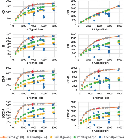
Results of human-yeast alignment. Each chart shows one evaluation measure (as detailed in Table 2). PrimAlign and its modifications were run to output the same num-ber of aligned pairs as other algorithms for direct comparison. The red cross marks denote the level of aligned pairs for PrimAlign using the default threshold (dark red––for U; light red––for W; they mostly overlap). U––unweighted networks, W––weighted networks

• For seven out of eight evaluation measures, PrimAlign exhibits a saturation curve typical for higher accuracy in more confident pairs for small outputs. This suggests that PrimAlign’s confidence score correlates with accuracy.

• The semantical measure GO as the only one results in a linear trend and is almost identical to other algorithms except for the aligners with enforced coverage, which shows lower semantical content and NETAL. This suggests that more confident pairs are not semantically more similar comparing to less confident pairs. However, it points towards inefficiencies in aligners with enforced coverage and NETAL.

• NETAL is an outlier, for which none of its aligned pairs was found among known orthologs, indicative of biologically incorrect alignment.

• Apart from GO, aligners with enforced coverage achieve lower scores across other evaluation measures as well. This is also an indicator of their low biological quality.

• Results for semantically weighted and unweighted networks on input are almost identical for all algorithms supporting weights except for NetworkBLAST, which shows a big difference in the number of aligned pairs (but similar cost measures). This might mean that semantical weighting does not provide valuable information for aligners.

• PrimAlign-Seq and PrimAlign-Topo also exhibit a saturation trend, although none of them reaches the score of PrimAlign. This suggests that both sequence similarity and network topology contribute towards the final power of PrimAlign.

• The default threshold of PrimAlign produces a reasonable number of aligned pairs across all three alignment tasks. This suggests that the default threshold is good for alignment of networks of various sizes and density. More detailed effects of changing the threshold are shown in Supplementary Information as Figure S3.

• PrimAlign outperforms other algorithms at their size of output with a statistical significance across all categories of evaluation measures, as shown in Table 4 for human-yeast alignment and Supplementary Tables S2a and S2b for the other alignment tasks.

  Table 4.

  Statistical comparison of PrimAlign with the others

  Aligner	Weighted	KO	GO	EN	IP	CE-F	CE-O	LCCC-F	LCCC-O
  AlignMCL	No					***	***	**	**
  AlignMCL	Yes					***	***	**	**
  AlignNemo	No	***	***	***	***	***	***	***	***
  AlignNemo	Yes	***	***	***	***	***	***	***	***
  CUFID	No	***	***	***	***	***	***	***	***
  CUFID	Yes	***	***	***	***	***	***	***	***
  HubAlign	No	***	***	***	***	***	***	***	***
  IsoRankN	No	***		***		***	***	***	***
  MAGNA++	No	***	***	***	***	***	***	***	***
  MI-GRAAL	No	NA	NA	NA	NA	NA	NA	NA	NA
  NETAL	No	***	***	***	***	***	***	***	***
  NetCoffee	No	***	***	***	***	***	***	***	***
  NetworkBLAST	No	***	***	***	***	***	***	***	***
  NetworkBLAST	Yes	***	***	***	***	***	***	***	***
  PINALOG	No	***	***	***	***	***	***	***	***
  SANA	No	***	***	***	***	***	***	***	***
  SMETANA	No	***	***	***	***	***	***	***	***
  SMETANA	Yes	***	***	***	***	***	***	***	***
  WAVE	No	***	***	***	***	***	***	***	***

  Notes: Statistical comparison of differences in evaluation measures between PrimAlign with unweighted networks on input and the other algorithms for human-yeast alignment. (empty field) P > 0.05

  *

  P ≤ 0.05

  **

  P ≤ 0.01

  ***

  P ≤ 0.001. Green = improvement.

• However, for the smallest alignment task, aligners with enforced coverage shows very high scores in combined topological measures although this is not accompanied with such an increase in other measures and not replicated in other alignment tasks. This could mean that these algorithms are overfitting with topological optimization and for such small networks with relatively few known orthologs the combined scores might be skewed towards the contribution of topological similarity.

• Results of KO, IN and EN measures tend to correlate even though their lists of orthologs differ and overlap only partially. This is not surprising, as we expect that all of them provide quality orthologs and that the measures should correlate with algorithms accuracy regardless of which sub-set of quality orthologs is used. Results of combined topological measures also correlate with each other, suggesting that when filtered for known orthologs, CE and LCCC are of similar evaluation power.

4.3 Results with synthetic networks

Results of all 30 runs with unweighted synthetic networks in terms of precision, recall, GS³ and NCV-GS³ are summarized in Figure 2. For PrimAlign and AlignMCL, the results are very similar across the measures at the same size of aligned pairs. By default, PrimAlign still outputs more confident pairs with mean precision above 70%, whereas AlignMCL produces pairs with precision around 55% in exchange for higher recall. SANA achieves mean precision around 45% even though its recall is also low. On the other hand, SANA scores well in topological measures GS³ and NCV-GS³. This corresponds with our previous tests and confirms the suspicion that SANA overfits alignment topology and produces biologically less precise predictions. Figure 3 shows precision-recall curve for PrimAlign together with locations of AlignMCL and SANA for the first synthetic network. Unfortunately, data of neither of these algorithms allow to construct their own precision-recall (p-r) curves, which would be the ideal case for comparison and statistical evaluation of their performance in terms of auPR (area under p-r curve).

Fig. 2.

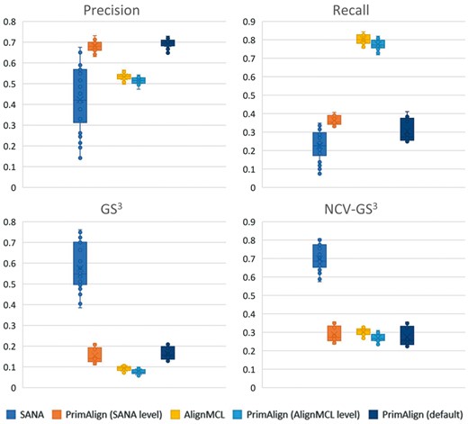
Results of tests with 30 synthetic networks. Comparing precision, recall and topological measures of PrimAlign with SANA and AlignMCL at their size of aligned node pairs

Fig. 3.

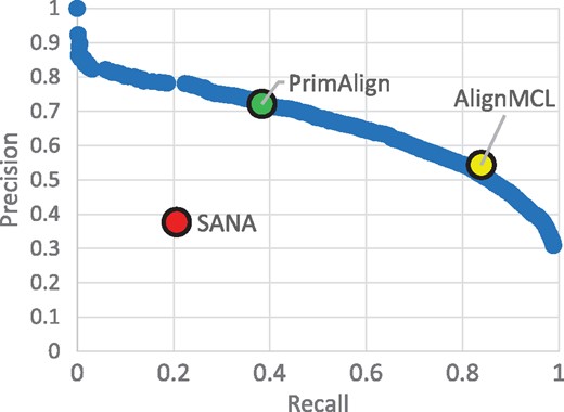
Example of P-R curve. P-R curve of PrimAlign for the 1st synthetic network compared with SANA and AlignMCL. The result of PrimAlign for the default threshold is highlighted.

4.4 Runtime comparison

Runtimes of individual algorithms are listed in Supplementary Table S5. NetCoffee is the fastest algorithm. However, its performance was shown to be poor, mostly worse than both restricted versions PrimAlign-Seq (which actually finishes within 1 second) and PrimAlign-Topo. PrimAlign was the only other algorithm running less than 1 minute for the largest alignment task, showing its great scalability. On the other side of the spectrum with runtime more than 1 hour are PINALOG, MAGNA++ (more than 10 hours), NetworkBLAST (more than 1 day), IsoRankN (more than 4 days) and MI-GRAAL (estimated 2 weeks of pre-processing for the smallest alignment task). As visible from runtime ratios between the tasks, some algorithms are very difficult to scale.

5 Conclusion

Biological network aligners pursue the goal of finding pairs of functionally matching proteins between the networks. This is still a task with incomplete information and needs to be solved heuristically. Some algorithms adopt the constraints of one-to-one alignment or complete coverage of proteins from the smaller network. (Neither one of them is biologically valid due to the gene duplications and other evolutionary mechanisms.) Other algorithms may use more subtle assumptions. Some of them perform subsequent grouping of aligned pairs into highly conserved clusters (local aligners). In each case, each algorithm has its own assumptions or heuristics to apply to recognize correct orthologs.

In this paper, we introduced PrimAlign, a new algorithm for pairwise global alignment of PPI networks, based on the Markovian representation and PageRank technique. PrimAlign performs global many-to-many alignment with asymptotic time complexity O(n), which is the theoretical minimum for this task, guaranteeing high scalability. The performance was evaluated on alignment tasks with three model species and compared to 14 prevalent network alignment algorithms. Various evaluation measures were used: ground-truth-based measures with data from two different orthology databases, annotation-based measures to evaluate functional and semantic consistency and topology-based measures combined with the previous measures. Adjusting the output size in terms of the number of aligned pairs allowed a direct comparison between PrimAlign and the other algorithms. Additional evaluation was performed with 30 synthetic networks and high performing representatives of global and local aligners.

As a result, the proposed method outperforms the other algorithms on real networks with statistically significant differences demonstrated for all evaluation measures except for the semantic similarity measure. This measure exhibits approximately the same trend across the algorithms, grows linearly with respect to the number of aligned pairs, and therefore, it seems to be of little value for evaluation. Furthermore, weighting PPI networks with semantic similarity seems to be of no benefit. The previous algorithm with closest results was AlignMCL. In the task with smallest and least dense networks, four other algorithms (SANA, WAVE, HubAlign and PINALOG) achieved significantly higher scores in combined topological evaluation measures. We speculated that this result sourced from high topological optimization of these algorithms and might not be biologically superior, indicated by non-superior scores in other categories and non-replicability in the alignment of larger networks.

Additional comparison with AlignMCL and SANA on synthetic networks, where true functional assignments are known, confirmed the case. Even though SANA achieved very high topological score, its real performance was poor with a high ratio of FPs as well as FNs. This result justifies our decision not to include topological scores among evaluation measures because of the suspicion that optimizing topology might easily result in overfitting and failing to correlate with functional conservation. Furthermore, AlignMCL performs very similarly to PrimAlign. However, AlignMCL produced relatively many aligned pairs, leading to lower precision in compromise to achieve higher recall, and there is no parameter to tune the confidence threshold, in contrary to PrimAlign. This also means that while PrimAlign can be evaluated with auPR, we cannot construct precision-recall curve for AlignMCL, even though auPR would be probably the most reasonable measure to statistically evaluate performance in synthetic networks.

The computation time of PrimAlign is excellent thanks to sparse computations. On the test machine, it runs faster comparing to other algorithms by 1–4 orders of magnitude, which makes it suitable for alignment of complex biological networks. Only NetCoffee was faster although it did not produce comparably good results. The source code of the proposed method, written in C# language, is available at http://web.ecs.baylor.edu/faculty/cho/PrimAlign. With less than 70 lines of code, it is probably the most compact and lightweight alignment algorithm available, it is easy to read and easy to be extended. The raw evaluation results and input files are also available.

Conflict of Interest: none declared.