Optimality and identification of dynamic models in systems biology: an inverse optimal control framework

Abstract

Motivation

Optimality principles have been used to explain many biological processes and systems. However, the functions being optimized are in general unknown a priori. Here we present an inverse optimal control framework for modeling dynamics in systems biology. The objective is to identify the underlying optimality principle from observed time-series data and simultaneously estimate unmeasured time-dependent inputs and time-invariant model parameters. As a special case, we also consider the problem of optimal simultaneous estimation of inputs and parameters from noisy data. After presenting a general statement of the inverse optimal control problem, and discussing special cases of interest, we outline numerical strategies which are scalable and robust.

Results

We discuss the existence, relevance and implications of identifiability issues in the above problems. We present a robust computational approach based on regularized cost functions and the use of suitable direct numerical methods based on the control-vector parameterization approach. To avoid convergence to local solutions, we make use of hybrid global-local methods. We illustrate the performance and capabilities of this approach with several challenging case studies, including simulated and real data. We pay particular attention to the computational scalability of our approach (with the objective of considering large numbers of inputs and states). We provide a software implementation of both the methods and the case studies.

Availability and implementation

The code used to obtain the results reported here is available at https://zenodo.org/record/1009541.

Supplementary information

Supplementary data are available at Bioinformatics online.

1 Introduction

Optimality principles in biology have a long history. The optimal design principle hypothesis was formally stated by Rashevsky (1961) and later extended by Rosen (1967). This principle claims that the biological structures necessary to perform a certain function must be of maximum simplicity, and optimal regarding energy and material requirements. Similar optimality principles have been shown to agree with observations about living matter at different levels of organization, from basic molecular and cell biology phenomena, up to the levels of organs, individuals, populations and their evolution (Alexander, 1996; Dekel and Alon, 2005; de Vos et al., 2013; Friston, 2010; McFarland, 1977; Parker et al., 1990; Popescu, 1998; Schaffer, 1983; Smith, 1978; Sutherland, 2005; Todorov, 2004). The general justification is that evolution by natural selection is the mechanism behind these optimality principles, a concept already present in Darwin’s work.

Sutherland (2005) claims that these optimality principles allow biology to move from merely explaining patterns or mechanisms to being able to make predictions from first principles. Bialek (2017) makes the important point that optimality hypotheses should not be adopted because of esthetic reasons, but as an approach that can be directly tested through quantitative experiments. Mathematical optimization could therefore be regarded as a fundamental research tool in bioinformatics and computational systems biology (Banga, 2008; de Vos et al., 2013; Ewald et al., 2017; Handl et al., 2007; Heinrich et al., 1991; Mendes and Kell, 1998).

Here we consider the role of optimality principles in molecular and cell biology. In particular, we focus on the problem of explaining and predicting dynamics at those levels based on optimality considerations. In the context of biochemical pathways, pioneering studies were performed in the 1990s considering optimization in metabolic networks (Hatzimanikatis et al., 1996; Heinrich et al., 1991, 1997; Heinrich and Schuster, 1996). To our knowledge, the first attempt to explain the dynamics in metabolic networks was presented by Klipp et al. (2002) considering linear networks and the hypothesis of minimum transition time. Interestingly, the predicted pattern of gene expression dynamics was later found experimentally (Zaslaver et al., 2004). Therefore, the pioneering work of Klipp et al. (2002) is a good example of the predictive value of optimality-based methods in systems biology.

Since then, several studies (Bartl et al., 2010; Oyarzún et al., 2009) recognized that the original question considered by Klipp et al. (2002) can be naturally formulated as an optimal control problem. Optimal control (also known as dynamic optimization when the system is open loop) considers the optimization of a dynamic system, that is, one seeks the optimal time-dependent input (open loop control) to minimize a certain performance index (cost function). In recent years, a number of studies have extended these ideas considering more realistic pathways (larger size and more complex topologies), and in some cases making use of increasingly sophisticated optimal control formulations (Bartl et al., 2013; de Hijas-Liste et al., 2014, 2015; Ewald et al., 2017; Nimmegeers et al., 2016; Oyarzún, 2011; Waldherr et al., 2015; Wessely et al., 2011). Similarly, Giordano et al. (2016) have recently used optimal control to obtain novel insights into microbial growth strategies, successfully explaining the dynamical allocation of cellular resources. Interestingly, these authors have also shown that a near-optimal control strategy based on a coarse-grained model exhibited structural similarities with the regulation of ribosomal protein synthesis in Escherichia coli.

These studies reflect the potential benefits and the increasing importance of applying control engineering concepts to systems and synthetic biology problems, an area that is still in its infancy (Doyle and Stelling, 2006; He et al., 2016; Wellstead et al., 2008). However, an open question in all these studies is that the cost function (i.e. the performance index being optimized) is unknown a priori. Although multiobjective dynamic optimization can be used to consider several objectives simultaneously (de Hijas-Liste et al., 2014), researchers still have to come up with cost functions describing the hypothetical underlying optimality principle.

It is important to note that these studies should be distinguished from the more standard application of optimal control to biosystems and bioprocesses. This is an area where a lot of research has been carried out, and it includes well known problems as e.g. how to operate a bioreactor to ensure optimal production of a substance of interest (Smets et al., 2004), or how to create or inhibit oscillations or patterns (Lebiedz and Brandt-Pollmann, 2003; Sootla et al., 2016). All these problems have pre-defined performance indexes, which are related to the optimal design and manipulation of biosystems by humans, i.e. the cost function is known a priori.

Here we consider the use of an inverse optimal control (IOC) perspective to find the optimality principle which can explain (and/or predict) dynamic behavior in biological systems. That is, we face the situation where the cost function is not known a priori. The usual approach so far has been to hypothesize and then test different cost functions for a given biosystem, i.e. computing the optimal control and checking, a posteriori, if there is a match between the predicted and the observed dynamics.

With the aim of finding a more systematic approach, we present here an IOC framework. Briefly speaking, IOC aims to find the optimality criteria that can explain a set of given dynamic measurements. In more detail, given a dynamic model of a biosystem with unknown parameters and time-series observations (measurements) of (at least part of) its dynamic states and (some or none) of the inputs, we seek to find the underlying optimality criteria (cost function or performance index) together with the unmeasured inputs and time-invariant model parameters that explain the measurements in the best way. This problem can also be regarded as estimating parameters in optimal control problems, and a number of important variants can be derived depending on what is measured.

2 Materials and methods

2.1 Approach

We consider two classes of IOC problems:

• IOCP-1—input reconstruction as an optimal tracking problem: given a non-linear dynamic model of a biosystem and a set of measurements (time-series data of observed states), find the time-dependent inputs and time-invariant parameters that explain the available time-series data.

• IOCP-2—general IOC problem: given a non-linear dynamic model of a biosystem operating with an underlying optimality principle, find the cost function, the time-dependent inputs and time-invariant parameters that explain the available data (time-series measurements).

Problem IOCP-1 can be regarded as a special case of problem IOCP-2. It should be noted that several other variants of IOCP-1 are possible, depending e.g. if the system is partially or fully observed. A few instances of this input reconstruction problem have been recently studied in the domains of systems biology (Kahm et al., 2012; Kaschek et al., 2016; Lang and Stelling, 2016; Schelker et al., 2012) and pharmacokinetics (Trägårdh et al., 2016, 2017). Particularly interesting variants of IOCP-1 have been presented by Engelhardt et al. (2016, 2017) to model biosystems with unknown inputs as well as missing and erroneous interactions. Here we are considering scenarios where all relevant inputs are known and there are no wrong interactions, showing that even under these assumptions the inverse problems can be extremely challenging due to lack of identifiability.

To the best of our knowledge, problem IOCP-2 has not been previously studied in systems biology, but it has recently received attention in the areas of robotics (Clever et al., 2016; Panchea and Ramdani, 2015) and biomechanics (Hatz et al., 2012; Hatz, 2014; Mombaur, 2016).

Next, we present the general problem statements, followed by a section detailing numerical strategies to solve them. We also discuss several important issues related to the structural identifiability of these problems.

2.2 Statement of the IOC problem

Here we consider dynamic models of biological systems given by sets of deterministic non-linear ordinary differential equations (ODEs). The systems are assumed to be at least partially observable, i.e. we can obtain time series measurements of at least some of the states. Here we do not consider the scenarios of errors in the model or unknown inputs.

For the more general problem (IOCP-2), we assume that there is optimality with respect to certain unknown criteria from a finite set of possibilities. Our aim is to find both the criteria and the model parameters that best explain the observed data. This IOC problem is formulated as a bi-level optimal control structure, consisting of an upper (or outer) and a lower (or inner) optimization problem. The outer problem corresponds to a simultaneous input and parameter estimation problem (as detailed in the Supplementary Material), where the time-invariant model parameters p and time-dependent inputs (e.g. stimuli) $\mathbf{u}\left(t\right)$ are computed so the model predictions y fit the observed data $\tilde{\mathbf{y}}$⁠. The inner problem corresponds to a multi-objective optimal control problem (see also Supplementary Material), where the optimal solution of the time-dependent inputs $\mathbf{u}\left(t\right)$ is computed as Pareto optimal controls for the set of optimality criteria considered. The general mathematical formulation of the IOC problem IOCP-2 considering free terminal time becomes:

$$\underset{\mathbf{u}\left(t\right),\mathbf{p},t_f}{\text{min}}{\mathrm{J}}_{\text{outer}}[\mathbf{x},\mathbf{u},\mathbf{p}]$$

(1)

Subject to:

$$\underset{\mathbf{u}\left(t\right),t_f}{\text{min}}{\mathbf{J}}_{\mathbf{i}\mathbf{n}\mathbf{n}\mathbf{e}\mathbf{r}}[\mathbf{x},\mathbf{u},\mathbf{p}]$$

(2)

Subject to:

$$\begin{array}{c}\frac{\mathrm{d}\mathbf{x}}{\mathrm{d}t}=\tilde{\mathbf{\Psi }}\left[\mathbf{x}\right(t,\mathbf{p}),\mathbf{u}(t),\mathbf{p},t],\hfill \\ \mathbf{x}(t_0,\mathbf{p})={\mathbf{x}}_0\hfill \end{array}$$

(3)

$$\mathbf{y}(\mathbf{x},\mathbf{p})=\mathbf{g}\left(\mathbf{x}\right(t,\mathbf{p}),\mathbf{p})$$

(4)

$$\mathit{\eta }\left[\mathbf{x}\right(t,\mathbf{p}),\mathbf{u}(t),\mathbf{p}]=0$$

(5)

$$\mathit{\zeta }\left[\mathbf{x}\right(t,\mathbf{p}),\mathbf{u}(t),\mathbf{p}]\le 0$$

(6)

$${\mathit{\eta }}_{\mathit{\iota }}\left[\mathbf{x}\right(t_{\iota },\mathbf{p}),\mathbf{u}(t_{\iota }),\mathbf{p}]=0$$

(7)

$${\mathit{\zeta }}_{\mathit{\iota }}\left[\mathbf{x}\right(t_{\iota },\mathbf{p}),\mathbf{u}(t_{\iota }),\mathbf{p}]\le 0$$

(8)

$${\mathbf{u}}^{\mathbf{L}}\le \mathbf{u}\left(t\right)\le {\mathbf{u}}^{\mathbf{U}}$$

(9)

$${\mathbf{p}}^{\mathbf{L}}\le \mathbf{p}\le {\mathbf{p}}^{\mathbf{U}}$$

(10)

where:

$$J_{\text{outer}}=\sum _{k=1}^{n_{\hspace{0.17em}\text{exp}\hspace{0.17em}}}\sum _{j=1}^{n_{obs}}\sum _{i=1}^{n_s}{w}_{ijk}{\left(y_{ijk}\right(\mathbf{x}(t_i,\mathbf{p}),\mathbf{p})-{\tilde{y}}_{ijk})}^2$$

(11)

$${\mathbf{J}}_{\mathbf{i}\mathbf{n}\mathbf{n}\mathbf{e}\mathbf{r}}[\mathbf{x},\mathbf{u},\mathbf{p}]={\left[\begin{array}{c}{J}_1,J_2,\dots ,J_N\end{array}\right]}^T$$

(12)

For J_i, (⁠$i\in [1,N]$⁠):

$$J_i[\mathbf{x},\mathbf{u},\mathbf{p}]={\Phi }_M^i\left[\mathbf{x}\right(t_f,\mathbf{p}),\mathbf{p}]+{\int }_{t_0}^{t_f}{\Phi }_L^i\left[\mathbf{x}\right(t,\mathbf{p}),\mathbf{u}(t),\mathbf{p}]$$

(13)

where $\tilde{\mathbf{\Psi }}$ is the right-hand side of the system’s dynamics $\frac{\mathrm{d}\mathbf{x}}{\mathrm{d}t}$ (here we are assuming deterministic non-linear dynamics given by ODEs) and equations 5–8 are algebraic constraints, including path equalities and inequalities (⁠$\mathit{\eta },\hspace{0.17em}\mathit{\zeta }$⁠), and time-point constraints (⁠${\mathit{\eta }}_{\mathit{\iota }},\hspace{0.17em}{\mathit{\zeta }}_{\mathit{\iota }}$⁠). Equations (9) and (10) correspond to the bounds on the controls (time-dependent inputs, stimuli) (u) and time-invariant parameters (p), respectively. The system observables (y) are defined through an observation functional of states and parameters $\mathbf{g}\left(\mathbf{x}\right(t,\mathbf{p}),\mathbf{p})$⁠. The upper cost function $J_{\text{outer}}$ can take form of weighted (w_ijk) least squares (as above), but alternatively can be described by a maximum likelihood function. The inner problem’s cost functional is a multi-objective functional considering the set of N possible optimality criteria to explore. In its general form, each objective function J_i in this set (⁠$i\in [1,N]$⁠) consists of a Mayer (⁠${\Phi }_M^i$⁠) and a Lagrange (⁠${\Phi }_L^i$⁠) term.

Problem IOCP-1 (input estimation) can be considered as a special case of the formulation above where the lower level optimal control problem is ignored. In other words, it results in a standard optimal control problem where one seeks the optimal input and model parameters that best explain the observed data. This formulation is very general and flexible, allowing us to consider problems with arbitrary inputs, multi-experimental settings and multiple criteria for the optimality hypothesis.

2.3 Solution strategy

The solution of the above bi-level formulation is extremely challenging. Here we transform this hierarchical IOC problem IOCP-2 into a sequence of two optimal control problems with a subsequent identification of the optimality principle using the set of Pareto optimal controls compatible with the system dynamics and the observed data. In other words, we solve the above bi-level formulation by decomposing it as follows:

• Step 1: we first solve the outer input estimation problem to obtain the time-dependent inputs ${\mathbf{u}}^{*}\left(t\right)$ and time-invariant parameters ${\mathbf{p}}^{*}$ which explain the data in terms of the outer cost function metric. This is a standard single-objective non-linear optimal control problem. Note that parameters need to be structurally identifiable in order to ensure a unique solution (see further discussion about identifiability below).

• Step 2: we then use parameters ${\mathbf{p}}^{*}$ obtained in the previous step to compute the Pareto set of optimal controls (inner problem). Note that this is a multi-objective non-linear optimal control problem.

• Step 3: finally, we find the solution located in the Pareto set which is consistent with the experimental data.

The corresponding workflow is shown in Figure 1. Note that for the case of IOCP-1, only Step 1 is necessary.

Fig. 1.

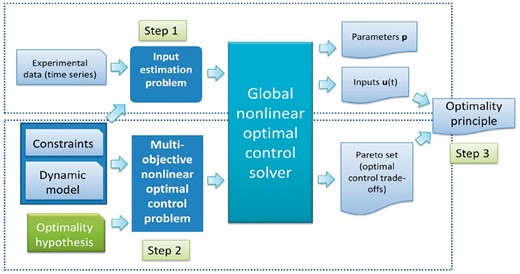
Overall workflow of the solution strategy for IOC problems

For the sake of completeness, the following considerations and numerical details were used to implement the above steps in an efficient way:

• The optimal control problem in Step 1 is a standard non-linear dynamic optimization problem. In the case of the multi-objective optimal control problem of Step 2, we use an epsilon-constraint decomposition to transform it into a set of single-objective optimal control problems. Thus both steps result in a set of non-linear optimal control problems.

• These non-linear optimal control problems are solved using the control-vector parameterization approach, CVP (Vassiliadis et al., 1994). The resulting non-linear programming problems are typically multimodal (Banga et al., 2005) so we use a hybrid global-local optimization method combining the enhanced Scatter Search (eSS) and efficient local solvers (Egea et al., 2009), as implemented in AMIGO2 (Balsa-Canto et al., 2016). More details are given in the Supplementary Material.

• Due to the ill-conditioning of these problems, regularization terms and/or constraints are used in the cost functions, as detailed below.

• It should be noted that our methodology can handle non-smooth or discontinuous dynamics thanks to the use of the global optimizer. This is illustrated with some of the examples below which have inequality path constraints that behave as state events.

2.3.1 Regularization of cost functions

Regularization methods can be successfully used to reduce ill-conditioning and avoid over-fitting (Gábor and Banga, 2015). Here we make use of regularized cost functions in order to reduce the ill-conditioning of the IOCPs. Thus, we extend the objective functions by adding regularization terms to incorporate problem-specific prior knowledge and/or constraints. In particular, we have implemented (i) a Tikhonov regularization scheme to incorporate possible prior knowledge about inputs and parameters, expressed as reference sets $({\mathbf{u}}_{\text{ref}},{\mathbf{p}}_{\text{ref}})$⁠; (ii) a penalty on the second order derivative of the estimated inputs to avoid wild oscillations and ensure convexity in the resulting input profiles. The resulting regularization terms are given by:

$$J_{\text{outer}}^{\text{reg}}=J_{\text{outer}}+R_u+R_p+R_{d2}$$

(14)

$$R_u=\alpha ·\frac{{\sum }_{i=1}^{n_u}({\mathbf{u}}_i(t)-{\mathbf{u}}_{i,\text{ref}}(t){)}^2}{n_u·t_f}$$

(15)

$$R_p=\beta ·\frac{{\sum }_{j=1}^{n_p}{(p_j-p_{j,\text{ref}})}^2}{n_p}$$

(16)

$$R_{d2}=\omega ·\sum _{i=1}^{n_u}{\int }_0^{t_f}\frac{d^2{\mathbf{u}}_i\left(t\right)}{d{t}^2}dt$$

(17)

where J_outer is the cost function, that is considered to be regularized, and α, β and ω are the regularization parameters, i.e. the weights balancing prior knowledge and information in the data. Although a number of regularization tuning methods have been developed to choose these weights, for the general non-linear case this tuning remains an open question (Gábor and Banga, 2015). Here, we have adopted an iterative re-optimization scheme, similar to that of the L-curve method, where these weights are reduced in each re-optimization. As shown in the case studies below, we have found that these regularization terms can be very helpful for the incorporation of prior knowledge regarding the qualitative behavior of the inputs. For instance, we might want to avoid wild oscillations in the recovered inputs, or to impose a certain behavior compatible with the biochemical mechanisms (e.g. a decreasing profile for any species being degraded).

2.3.2 Implementation

The code implementing the case studies reported here is available at https://zenodo.org/record/1009541. This code makes use of the above numerical strategy, which has been implemented as a software (add-on) module for the AMIGO2 toolbox (Balsa-Canto et al., 2016). This new IOC add-on is available at https://sites.google.com/site/amigo2toolbox/home/amigo2_ioc. In all the computations reported here, we have used the eSS optimizer, a hybrid global-local optimization meta-heuristic available in AMIGO2.

2.4 Remarks about identifiability

Identifiability considers the possibility of uniquely inferring model parameters from experimental data (Walter and Pronzato, 1997). A model is structurally identifiable if it is theoretically possible to estimate its parameters under the ideal scenario of continuous noise free data. A model is identifiable in practice if (i) it is structurally identifiable, and (ii) we have sufficiently rich experimental data to achieve high-quality parameter estimates.

This fundamental question becomes even more relevant in the case of IOCPs, where we seek the simultaneous identification of parameters and time-dependent inputs. The latter will in general imply the addition of further degrees of freedom, thus inducing lack of structural identifiability. We illustrate this in Figure 2 with a simple example regarding the reaction $X_1\stackrel{u,k_1}{\to }{X}_2\stackrel{k_2}{\to }$ which involves an inducer concentration, u. The reactant X₁ is present in excess, therefore we assume that its concentration x₁ is known and constant throughout the process. We can observe x₂ dynamics. The production and degradation rates have kinetic parameters k₁ and k₂. We considered a simple case in which u follows an exponential decay, $u\left(t\right)=k_u{e}^{-k_{t}t}$⁠. Figure 2 illustrates how different combinations of k₁ and k_u produce exactly the same x₂ profile for the same value of the product $k_1{k}_u$⁠. In other words, for this simple example, it will not be possible to individually identify k₁ and k_u but only their product. Other illustrative examples can be found in the Supplementary Material.

Fig. 2.

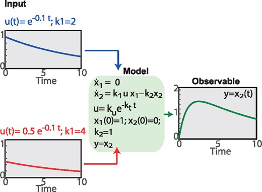
Illustrative example of lack of structural identifiability in IOCP. The figure shows a forward problem where two different input profiles (k_u = 1 and $k_u=0.5$⁠, with $u(t)=k_u\hspace{0.17em}\text{exp}(-0.1t)$⁠) result in the same output y. Thus, if we attempt to solve the inverse problem using observations of this output y, it will not be possible to uniquely recover the input, even for the ideal case of continuous noise-free measurements of the output

Assessing the structural identifiability of a non-linear dynamic model can be a rather complicated task. The analysis requires symbolic manipulation, which may become computationally prohibitive (Chis et al., 2011b). Trägårdh et al. (2017) is one of the few studies that has considered identifiability in an input estimation problem, analyzing parametric and stimuli structural identifiability separately. Here we have considered alternative possibilities to assess the identifiability of the IOCP formulation presented above. Since the structural identifiability of the general IOCP is (to the best of our knowledge) an open question, we have considered special cases where we could exploit the possibilities offered by methods developed in the context of parameter estimation (Chis et al., 2011b). For example, a Taylor series approach can be applied by either using time-dependent control parameterizations, or by assuming that the successive time derivatives of the stimuli (as evaluated at $t=0^{+}$⁠) are unknown parameters to be considered simultaneously alongside the model parameters p. Also, we can apply the generating series approach as implemented in GenSSI (Chis et al., 2011a), provided the stimuli are parametrized using continuous bounded functions of time. We illustrate the use of both approaches in the Supplementary Material.

2.5 Remarks about the reconstruction of the optimality principles

Although optimality principles have been studied at different levels of organization of biological systems, the case of metabolic networks deserves special attention. Heinrich et al. (1991) reviewed this topic in the early 1990s, stating several key ideas. First, the structural design and functioning of these networks are the outcome of evolution, which can be considered an optimization process. Second, the optimality assumption for these systems is supported by the fact that experimental perturbations (e.g. mutations) typically result in worse function. Third, the cost functions more frequently used were (i) maximization of fluxes, (ii) minimization of the concentration of metabolic intermediates, (iii) minimization of transient times, (iv) maximization of the sensitivity to external signals and (v) maximization of thermodynamic efficiencies. It should be noted that at that time most studies were restricted to stationary states.

Later, Klipp et al. (2002) explicitly considered dynamics and used the concept of minimum transition time to derive optimal temporal gene expression profiles, based on the assumption that cells have developed optimal adaptation strategies as an evolutionary response to changing environmental conditions. Notably, these predictions were experimentally confirmed by Zaslaver et al. (2004) for linear pathways, and agreed with earlier experimental observations. A detailed account can be found in Bartl et al. (2010), who make the case for a closely related cost function, the minimization of the operation time of substrate to product conversion, with an upper bound on the total amount of enzymes at any given time. These authors show how this alternative cost produces the same temporal pattern in linear pathways (just-in-time expression), while still being consistent with the assumption that high fitness requires high flux.

Although the vast majority of studies in this field have considered single cost functions, it is interesting to realize that Heinrich et al. (1991) had already suggested the use of multicriteria optimality, a concept further motivated in their later book (Heinrich and Schuster, 1996). The motivation was based on the idea that appropriate objective functions must be used to evaluate the efficiency (fitness) of a given system, and that it is very unlikely that the structure and dynamic behavior of current metabolic networks can be explained on the basis of a single objective, especially considering their many biological functions and the interactions between them. To the best of our knowledge, de Hijas-Liste et al. (2014) were the first to use multicriteria optimal control in the context of metabolic pathways, predicting the full set of best trade-offs (known as the Pareto set) between conflicting objectives.

Here we adopt this multicriteria view for the inverse problem of finding the underlying optimality principles. The method presented above for the general IOCP-2 problem starts from a list of candidate cost functions, and aims to find the point in the Pareto set which agrees with the experimental data and where the reconstructed inputs agree with the observed ones (although the latter are not used in the solution of the inverse problem).

3 Results

We present results for several challenging case studies. We first consider a problem of input estimation (IOCP-1). A second, more challenging problem of the same class is presented in the Supplementary Material to illustrate the scalability of the method regarding the IOCP-1 class. Next we present two instances of the more general IOC problem (IOCP-2). Simulated data (i.e. pseudo experimental data generated by simulation with different noise levels) are used in order to better assess the methodology. In these scenarios using simulated data, the true input functions (and optimality criteria, in the case of IOCP-2) are known and therefore we can carefully analyze the performance and accuracy of the method. However, it should be noted that in two cases we also consider scenarios with real data. The goodness of fit is evaluated using the normalized root mean square error (NRMSE; more details and other metrics in the Supplementary Material). All the computations were carried out on a PC Intel Xeon E5-2630@2.30 GHz using Matlab R2015B under Windows 7.

3.1 Case study JAK-STAT: input reconstruction for the JAK2-STAT5 signaling pathway

This case study is an example of IOCP-1, based on the problem considered by Schelker et al. (2012), where we seek the simultaneous input reconstruction and parameter estimation in a dynamic model of the JAK2-STAT5 signaling pathway. The detailed mathematical statement is given in the Supplementary Material. The problem has one time-dependent stimulus (pEpoR, which is treated as unknown here), nine internal state variables and two observables. Real measurements are available for both the observables and the stimulus. Our aim here is to simultaneously estimate the model parameters and the time-dependent trajectory for the input (stimulus), using only the experimental data for the observables in the cost function. The estimated input is then compared with the (unused) measurements of pEpoR. In other words, we only use the pEpoR measurements for the a posteriori analysis of the goodness of the input estimation.

This example is well suited to illustrate the importance of identifiability analysis in this class of problems. We provide a detailed structural identifiability analysis in the Supplementary Material, revealing that it is not possible to uniquely and simultaneously estimate all model parameters and pEpoR(t). In particular, p₁, p₄ and the scaling parameters are structurally non-identifiable. Based on this, we considered the problem of estimating $p_{2-3}$⁠, the offsets and pEpoR(t). Scaling parameters were fixed to nominal values. A piecewise linear approximation for the input pEpoR(t) was considered. Based on the nature of the stimulus, we used regularization to avoid wild oscillatory behavior and over-fitting (i.e. fitting the noise instead of the signal). The results are depicted in Figure 3, showing a good agreement (NRMSE = 0.142) between the estimated input and the input measurements (not used in our method), and a very good fit of the model predictions to the observed states measurements (NRMSE = 0.084). Computation times were in the range of 1–4 min.

Fig. 3.

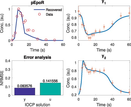
Case study JAK-STAT: estimated versus measured input (pEpoR) profiles, along with the fit for the two observables (y₁ and y₂). The lower left subfigure shows the goodness of the estimation as measured by the NRMSE with respect to the observables (y) and the input (u)

In the Supplementary Material, we include detailed results for two additional scenarios: (i) a subcase considering the ideal scenario of synthetic noiseless data, for which we achieve almost perfect estimations for both inputs and parameters, and (ii) a subcase using synthetic data generated with the addition of 5% heteroscedastic proportional noise.

3.2 Case study LPN3B: linear pathway with three enzymatic reactions

This is a first example of the more general IOCP-2 problem class, where we seek to identify the underlying optimality criteria along with the time-dependent stimuli and the time-invariant parameters considering a metabolic pathway model. This problem is a generalization of the dynamic optimization problem considered by de Hijas-Liste et al. (2014), based on the study by Bartl et al. (2010). In brief, we consider a linear chain of enzymatic reactions where the hypothesis is that the time-dependent enzyme concentrations correspond to an optimal trade-off between minimum conversion time and minimum accumulation of intermediates. The corresponding Pareto front is shown in Figure 4. We take the upper left (circled) point as reference, and generate pseudo-experimental data for those conditions. Then we consider the inverse problem of recovering the inputs and the optimality trade-off from the data. From an optimal control perspective, this case study is computationally challenging due to its multimodality and the presence of algebraic path constraints on the states and the stimuli. We have assumed that the system is fully observed, and we generated pseudo-experimental data for two subcases: LPN3B0 (noiseless data) and LPN3B10 (data with 10% heteroscedastic proportional noise). The detailed mathematical statement is given in the Supplementary Material.

Fig. 4.

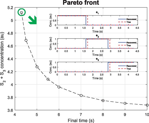
Case study LPN3B10: Pareto front (optimal trade-offs for the cost functions) indicated the reference point selected for the IOCP-2 problem. The good agreement between estimated and true inputs is shown in the figure inset. The error of the estimation is ${\text{NRMSE}}_y=0.13$ and ${\text{NRMSE}}_u=0.14$

First, we performed a structural identifiability analysis, revealing that it is not possible to simultaneously and uniquely estimate the kinetic constants and the time-dependent enzyme profiles. We also confirmed this property numerically, i.e. we were able to obtain different combinations of enzyme activation profiles and kinetic parameters which result in the same good fit to the data (full details of these identifiability issues are given in the Supplementary Material).

Next, in order to handle this lack of structural identifiability, we used prior knowledge so as to enforce a unique numerical solution. This prior information was embedded into the regularization scheme and the selected bounds. We also considered several types of control parameterizations for the inputs (enzyme activation profiles). We achieved a very good reconstruction of the original stimuli trajectories and the parameter values in both subcases. The goodness of the input estimation for the noisy subcase is given in Figure 4, showing a recovered just-in-time activation profile in good agreement with the true one (not used in the reconstruction). Note that the corresponding NRMSE of 14% is due to the small shifts in the switching times. Computation times were in the range of 1–20 min. Further details for both subcases can be found in the Supplementary Material.

3.3 Case study SC: central metabolism of Saccharomyces cerevisiae during diauxic shift

As a second example of problem IOCP-2, we considered the dynamics of the central metabolism of yeast during diauxic shift in a nutrient depletion scenario. Our formulation is based on the problems studied by Klipp et al. (2002) and de Hijas-Liste et al. (2014), where the model considers six reactions: upper and lower glycolysis, ethanol formation and ethanol consumption, the TCA cycle and the respiratory chain. This description results in 9 dynamic states, 8 parameters and six time-dependent enzyme concentrations. In the previous study by de Hijas-Liste et al. (2014), the objective was to find the enzyme activation profiles so as to compute the Pareto set of optimal control considering two objective functions (survival time and enzyme synthesis cost). A path inequality constraint is used to ensure that concentrations of NADH and ATP remain above critical values at all times. In other words, Pareto-optimal enzyme profiles were computed which ensure long-term homeostasis of key metabolites under conditions of a diauxic shift.

Here, we formulate a synthetic problem by selecting a reference point in the Pareto front and considering the full IOC problem: given synthetic time-series data for the observed states at such a reference point, estimate the model parameters, the inputs (enzyme time-dependent activation profiles) and the optimality criteria which best explain such data.

This case study is more complex than LPN3B, including more time-dependent stimuli and several challenging path constraints on the concentrations of NADH and ATP. The detailed mathematical formulation and a diagram of the network are given in the Supplementary Material. We considered two different subcases based on the generated synthetic data: SC0 (noiseless) and SC10 (noisy, with 10% heteroscedastic proportional noise). Note that this case study is particularly interesting because real experimental data are also available, allowing qualitative comparisons (Klipp et al., 2002).

As expected, the problem is very ill-conditioned and exhibits identifiability issues of a similar nature to those in Section 3.2. The controls e_i appear only multiplying the parameters, making both of them structurally unidentifiable. Therefore, to reduce the identifiability issues, we re-formulated the model, estimating the products of parameters and stimuli (details in the Supplementary Material). This re-formulated problem has nine dynamic states, two parameters and six time-dependent products of enzyme concentrations and kinetic parameters which we consider as our new inputs.

The results for the noiseless subcase SC0 are given in the Supplementary Material, showing a very good reconstruction of the inputs (⁠${\text{NRMSE}}_u=0.2$⁠) and an almost perfect fit to the data (⁠${\text{NRMSE}}_y=0.001$⁠). The more realistic SC10 subcase was also successfully solved, showing that despite the 10% noise, our methodology was able to find a very reasonable reconstruction of the inputs (⁠${\text{NRMSE}}_u=0.29$⁠), and therefore a good identification of the optimality trade-off explaining the dynamics. In Figure 5 we show the matching between the estimated and the true input values, the corresponding fit of the estimated states to the data and the NRMSE values. Computation times were in the range of 15–90 min.

Fig. 5.

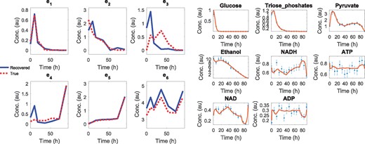
Case study SC: estimated versus true input values (left; NRMSE = 0.29), and the corresponding fit to observed data (right; NRMSE = 0.13), for the SC10 (10% noise) subcase

It is worth discussing the biological meaning of the estimated states and inputs. At early times, enzyme e₁ shows a peak of activity which allows the rapid consumption of glucose. Enzyme e₂ and e₃ also present significant activity at early times, resulting in the production of ethanol while glucose is still present. Later on, e₄ increases its activity, so ethanol is consumed to maintain the required levels of NADH and ATP. These results are consistent with the observed behavior of diauxic shift of yeast under glucose starvation conditions. An additional qualitative comparison with experimental data is given in the Supplementary Material.

4 Conclusions

Here we consider the question of systematically inferring optimality principles in cellular pathways from noisy dynamic data. We present a general IOC framework to address this question, where the objective is to simultaneously identify the underlying optimality principle, as well as the time-dependent inputs and time-invariant model parameters. We present a solution strategy where the IOCP is decomposed into an optimal tracking problem and a multi-criteria optimal control problem. As a special case, we also consider the subproblem of input and parameter estimation from noisy data.

Importantly, we discuss the existence and implications (in terms of fundamental limitations) of structural identifiability issues in the above problems. Further, we present a robust computational solution strategy based on regularized cost functions and the use of suitable direct numerical methods based on the control-vector parameterization approach. To avoid convergence to local solutions, we make use of hybrid global-local optimization methods.

We illustrate the performance of this framework by successfully solving several challenging case studies dealing with biochemical pathways of increasing size and complexity, including scenarios with simulated and real data. We highlight the importance of analyzing the structural identifiability issues present in these problems. We show how the limitations arising from these issues can be surmounted by model reformulation and/or the exploitation of prior knowledge. Similarly, practical identifiability issues (due to lack of information in the data) could be surmounted by incorporating more informative experiments and/or by performing model-reduction. Finally, we find that the methodology exhibits a satisfactory scalability in terms of computational cost as a function of problem size (details are provided in the Supplementary Material). It should be noted that large speedups could be obtained by exploiting the inherent parallelism of the methodology.

Funding

This research was supported by the European Union’s Horizon 2020 research and innovation program under grant agreement No 675585 (MSCA ITN ‘SyMBioSys’) and from the Spanish MINECO/FEDER projects SYNBIOFACTORY [grant number DPI2014-55276-C5-2-R], SYNBIOCONTROL [DPI2017-82896-C2-2-R] and IMPROWINE [grant number AGL2015-67504-C3-2-R]. N.T. is a MSCA ESR at IIM-CSIC (Spain).

Conflict of Interest: none declared.