DeepSol: a deep learning framework for sequence-based protein solubility prediction

Abstract

Motivation

Protein solubility plays a vital role in pharmaceutical research and production yield. For a given protein, the extent of its solubility can represent the quality of its function, and is ultimately defined by its sequence. Thus, it is imperative to develop novel, highly accurate in silico sequence-based protein solubility predictors. In this work we propose, DeepSol, a novel Deep Learning-based protein solubility predictor. The backbone of our framework is a convolutional neural network that exploits k-mer structure and additional sequence and structural features extracted from the protein sequence.

Results

DeepSol outperformed all known sequence-based state-of-the-art solubility prediction methods and attained an accuracy of 0.77 and Matthew’s correlation coefficient of 0.55. The superior prediction accuracy of DeepSol allows to screen for sequences with enhanced production capacity and can more reliably predict solubility of novel proteins.

Availability and implementation

DeepSol’s best performing models and results are publicly deposited at https://doi.org/10.5281/zenodo.1162886 (Khurana and Mall, 2018).

Supplementary information

Supplementary data are available at Bioinformatics online.

1 Introduction

The heterologous expression of proteins in standard host cells, such as Escherichia coli, often render the proteins insoluble reducing their manufacturability (Chang et al., 2014). However, the exploration of structural and functional proteomics requires proteins to be produced in soluble form (Chan et al., 2010). Thus, solubility of proteins is crucial for production of proteins in both the pharmaceutical and research setting. Enhancement in protein solubility is usually attained by the use of weak promotors or strong denaturants followed by refolding (Davis et al., 1999), lower temperatures (Idicula-Thomas and Balaji, 2005), or optimization of other expression conditions (Magnan et al., 2009) such as codon optimization (van den Berg et al., 2012).

The primary structure plays a major role in determining the solubility of a protein. Previous studies (Bertone et al., 2001; Christendat et al., 2000; Davis et al., 1999; Idicula-Thomas and Balaji, 2005; Pédelacq et al., 2002; Trainor et al., 2017; Wilkinson and Harrison, 1991) indicated that several sequence-based features, such as the extent of charged and turn-forming amino acid residues, the level of hydrophobic stretches, protein folding and the length of the protein sequence, exhibit a strong association with the protein solubility. Several machine learning-based bioinformatics tools have been developed for protein solubility prediction to determine the soluble proteins in silico and omit the expensive trial and error procedures involved in wet-labs. These sequence-based predictors include PaRSnIP (Rawi et al., 2017), PROSO II (Smialowski et al., 2012), CCSOL (Agostini et al., 2012), SOLpro (Magnan et al., 2009), PROSO (Smialowski et al., 2007), RPSP (Wilkinson and Harrison, 1991) and the scoring card method (SCM) (Huang et al., 2012). The majority of these tools use a support vector machine (SVM) (Cortes and Vapnik, 1995; Suykens et al., 2002) as the core discriminative model on biologically relevant handcrafted features from the protein sequences to distinguish between the soluble and insoluble proteins. The recently proposed technique, PaRSnIP, uses a gradient boosting machine (GBM) (Friedman, 2001) on a dataset of over 8000 mono-, di- and tri-peptide frequency based features along with an additional 57 sequence and structural features. PaRSnIP identified that higher fractions of exposed residues positively correlate with protein solubility and tri-peptide stretches that contain multiple histidines negatively correlate with protein solubility. PROSO II utilizes a Parzen window model with a modified Cauchy kernel and a two-level logistic classifier. CCSOL uses an SVM classifier and identifies coil/disorder, hydrophobicity, β-sheet and α-helix propensities as primary differentiating features. SOLpro also uses a two-stage SVM to build the protein solubility predictor. The PROSO tool uses an SVM with an RBF (radial basis function) kernel (Suykens et al., 2002) and a second-level Naive Bayes classifier. RPSP performs classification with a standard Gaussian distribution to distinguish soluble proteins from insoluble ones. Finally, the SCM method uses a scoring card by utilizing only dipeptide composition to estimate solubility scores of sequences.

The majority of these tools perform a two-stage classification using a plethora of sequence-based features including mono-, di- and tri-peptide frequencies i.e. over 8000 features. In the first stage, these methods perform a feature selection task to reduce the risk of over-fitting, followed by the discriminative classification step in the second stage. On the other hand, PaRSnIP relies on the feature importance scores from the GBM model to identify and prune the non-essential features.

In this study, our goal is to build a single-stage protein solubility prediction system that outperforms all existing sequence-based tools. We used Deep Learning models to identify the relationship between the k-mer structure in the input protein sequence and the solubility of the protein. We used convolutional neural networks (CNNs) (LeCun et al., 1995) to exploit the k-mer structure. CNNs construct non-linear high-dimensional k-mer vector spaces. These vector spaces enable the model to encode more information about the k-mer structure, necessary for predicting protein solubility, than just the k-mer frequencies as encoded in the feature vectors of previous machine learning techniques. Our work is inspired by the recent success of several research groups using Deep Learning to model protein sequences for secondary structure (SS) (Li and Yu, 2016; Wang et al., 2016) and residue-residue contact prediction (Wang et al., 2017). The main contributions of this article are:

• Our Deep Learning model can be applied directly to raw protein sequences without any extensive feature engineering, which is the hallmark of previous works. Applied directly to raw sequences, our model (DeepSol S1) attains comparable performance to the current state-of-the-art protein solubility predictor, PaRSnIP. Apart from mono-, di- and tri-peptide frequency features, both PaRSnIP and PROSO II use additional biological features extracted using various external feature extraction toolkits from the protein sequences. However, in Deep Learning framework, discriminative features are extracted from the raw input sequence while optimizing the model for predicting solubility. Hence, the feature representations learned by a Deep Learning model encode not just k-mer frequencies but also higher-level abstract structural features that are necessary for solubility prediction.

• Our proposed framework simplifies the solubility prediction work-flow for bioinformatics researchers by obviating the need for extensive feature engineering. By including the 57 biological features used in PaRSnIP, the Deep Learning model outperforms all the state-of-the-art sequence-based protein solubility predictors.

• Our DeepSol models are publicly available, permitting future extensions.

On an independent test set (Chang et al., 2014), we showed that our predictor, DeepSol, is at least 3.5% more accurate than PaRSnIP and at least 15% more accurate than second-best solubility predictor PROSO II. Furthermore, DeepSol was superior to all the current sequence-based protein solubility predictors on several other quality metrics including Mathew’s correlation co-efficient (MCC), selectivity and gain for soluble, and sensitivity for insoluble proteins. DeepSol is freely available at https://zenodo.org/record/1162886 (Khurana and Mall, 2018).

2 Materials and methods

2.1 Overview

The problem of protein solubility prediction is a binary classification problem. We learn a mapping function that takes as input some parametrization, x, of a protein sequence and outputs a score in the range $[0,1]\in ℝ$ i.e. $t:\mathbf{x}\to [0,1]$⁠, where t is the mapping function. In this work, t is a CNN, a sparse variation of a feed-forward Neural Network architecture that exploits the co-occurrence patterns in the input. Protein sequence, is parametrized by a sequence of vectors, $\mathbf{x}=(x_1,x_2,\dots ,x_L)$⁠, where x_l is the one-hot encoded vector (Harris and Harris, 2010) i.e. a binary vector of length 21 (20 for amino acids and 1 for gap) with 1 bit active for the lth amino acid in the protein sequence. This is a common type of word or character encoding that is well known and widely used in natural language processing applications (Mikolov et al., 2013). Here L represents the fixed length of the protein sequence i.e. L = 1, 200.

2.2 Data partitioning

We used an initial training dataset consisting of 58 689 soluble and 70 954 insoluble protein sequences originally compiled in (Smialowski et al., 2012). We then performed two major preprocessing steps as utilized in PaRSnIP (Rawi et al., 2017) to avoid any unwanted bias and to ensure heterogeneity of sequences within the training set. Similar to previous work (Agostini et al., 2012; Smialowski et al., 2012), we first used CD-HIT (Fu et al., 2012; Li and Godzik, 2006) to decrease sequence redundancy within the training data with a maximum sequence identity of 90%. Second, we pruned out all sequences from the training set that had a sequence identity ≥30% to any sequence in the independent test set to prevent any bias caused by homologous sequences. The final training data included 28 972 soluble and 40 448 insoluble proteins.

The independent test set consisted of 1000 soluble and 1001 insoluble protein sequences first collected by (Chang et al., 2014). We employed this test set as a benchmark for a comprehensive comparison of several state-of-the-art sequence-based protein solubility predictors.

2.3 Data representation

2.3.1 Deep learning model input

The raw protein sequence was used as the input to the CNN. We did not perform any explicit feature engineering; the CNN was allowed to learn feature representations that best encode the information essential for solubility prediction.

2.3.2 Additional features

We used two sets of biological features (see Table 1); First, sequence-based features, such as the length of sequence, molecular weight and absolute charge were estimated along with features like the aliphatic indices (AIs), the average of hydropathicity (GRAVY), as well as fraction of turn-forming residues. Second, structural features predicted from the protein sequence using SCRATCH (Magnan and Baldi, 2014) were used. We determined three- and eight-state SS using SCRATCH to calculate the fraction of residues belonging to each class for a given protein sequence. Additionally, we estimated the fraction of exposed residues (FER) at different relative solvent accessibility (RSA) cutoffs. We used 20 different RSA cutoffs ranging from 0 to 95% with an interval of 5%. We also multiplied the FER by the hydrophobicity indices of the exposed residues. In total, we included 57 sequence and structural features in addition to the feature representations obtained from CNN to enhance the predictive capability of DeepSol.

Table 1.

Fifty-seven additional sequence and structural features for DeepSol

Sequence features	Structural features
Sequence length (1)	Three-state SS (3)
Molecular weight (1)	Eight-state SS (8)
Fraction turn-forming residues (1)	FERs
AI (1)	(0–95% cutoffs) (20)
Average hydropathicity (1)	FERs × hydrophobicity of exposed residues (0–95% cutoffs) (20)
Absolute charge (1)

Note: The number of features for each type is shown in parentheses.

2.4 Model

DeepSol consists of a CNN with multiple convolution blocks that maps the raw protein sequence to a fixed-dimensional continuous feature vector representation (Fig. 1b). The model is trained in a supervised learning setting (see Section 2.5) to ensure that the feature vector is discriminative for the classification task.

Fig. 1.

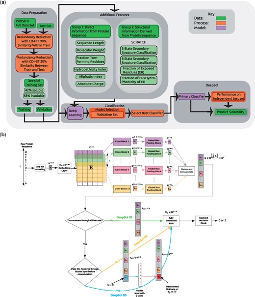
DeepSol overall framework. (a) DeepSol development flowchart. (b) The Deep Learning module is expanded to outline our proposed DeepSol architectures.Model Setting 1 (DeepSol S1) corresponds to the setting where continuous feature representation (h) of the raw input sequence, is the output of the K convolution and global max-pooling blocks. Convolution blocks are given by the set of triplets ${\{(f_k,q_k,a_k)\}}_{k=1\hspace{0.17em}\text{to}\hspace{0.17em}K}$⁠, where f_k is the convolution filter size, q_k is the number of convolutional filters and a_k is the activation function of the block (see Fig. 2 for details of the convolution block). In model Setting 2 (DeepSol S2), we concatenate h with 57 sequence and structural features (biological features referred as b), extracted using third-party bioinformatics tools. In model Setting 3 (DeepSol S3), we transform biological features using a feed-forward neural network to get ${\mathbf{b}}_p$ before concatenating with h

The input protein sequence, $\mathbf{x}\in {ℝ}^{L\times 21}$⁠, where 21 is the size of the amino acid symbol dictionary, is transformed to a fixed vector ${\mathbf{h}}_{\text{new}}\in {ℝ}^{d\prime }$ by performing the following transformations on x:

• Embed: x is projected to a dense continuous vector space by performing the transformation, $\mathbf{E}=\mathbf{x}{\mathbf{W}}_{\mathbf{e}}$⁠, where ${\mathbf{W}}_{\mathbf{e}}\in {ℝ}^{21\times e}$ is the embedding weight matrix, e corresponds to the embedding dimension and $\mathbf{E}\in {ℝ}^{L\times e}$ is the embedding matrix.

• Multi-convolution-pooling: The embedding matrix, E, is convolved with K parallel convolution blocks (see Fig. 1b). Convolution blocks are represented by a set of triplets ${\{(f_k,q_k,a_k)\}}_{k=\mathrm{1\dots }K}$⁠, where f_k is the convolution filter size, q_k is the number of convolution filters in the convolution block k and a_k is the activation function associated with that convolution block. We perform one dimensional convolution along the protein sequence length, L (see Fig. 2 for the description of a convolution block). Convolution blocks output a set of feature maps, ${\{Z_k\in {ℝ}^{(L-f_k+1)\times q_k}\}}_{k=1\hspace{0.17em}to\hspace{0.17em}K}$⁠. A convolution block k can be expressed using the following mathematical equation:

  $${\mathbf{Z}}_{\mathbf{k}}(m,q)=a_k\left(\sum _{i=0}^e\sum _{j=0}^{f_k}\mathbf{C}(i,j,q)\times \mathbf{E}(i,m+j)\right)$$

  (1)

  where, $q=1,\hspace{0.17em}\dots ,\hspace{0.17em}{q}_k,\hspace{0.17em}\mathbf{C}\in {ℝ}^{e\times f_k\times q_k}$ is the weight tensor that contains all the q_k convolution filters in that convolution block, a_k is the activation function; we use rectified linear unit (ReLU) (Xu et al., 2015) as the activation and ${\mathbf{Z}}_{\mathbf{k}}(m,q)$ is the $(m,q)$th element of the feature map ${\mathbf{Z}}_{\mathbf{k}}$⁠. The weight tensor C is learned during the training phase.  After obtaining each feature map, ${\mathbf{Z}}_{\mathbf{k}}$⁠, we carry out a global max-pooling operation. By performing max pooling, we prevent over-fitting by reducing the number of features during the training phase. This operation leads to a vector, ${\mathbf{h}}_k$ of dimension q_k. The vector ${\mathbf{h}}_k$ is obtained by:

  $${\mathbf{h}}_k=[\max {\mathbf{Z}}_{\mathbf{k}}(:,1);\max {\mathbf{Z}}_{\mathbf{k}}(:,2);\dots ;\max {\mathbf{Z}}_{\mathbf{k}}(:,q_k)]$$

  Finally, we concatenate all such ${\mathbf{h}}_k$ for $k=1,\dots ,K$ to get:

  $$\mathbf{h}=[{\mathbf{h}}_1;{\mathbf{h}}_2;\dots ;{\mathbf{h}}_K]$$

  We next describe the additional steps required to obtain the protein solubility prediction from the model.

• Biological feature concatenation: Three different experimental settings have been applied:

  • DeepSol S1: We simply use h for classification without the additional biological features, i.e. ${\mathbf{h}}_{\text{new}}=\mathbf{h}$⁠.

  • DeepSol S2: We concatenate the biological feature vector b, with h from the previous stage, to get ${\mathbf{h}}_{\text{new}}=[\mathbf{h};\mathbf{b}]$⁠.

  • DeepSol S3: We transform the biological features using a feed-forward neural network with p hidden units to obtain feature vector ${\mathbf{b}}_p\in {ℝ}^p$ and then concatenate it with h, to get ${\mathbf{h}}_{\text{new}}=[\mathbf{h};{\mathbf{b}}_p]$⁠.

    Here ${\mathbf{h}}_{\text{new}}\in {ℝ}^{d\prime }$ and all model settings are illustrated in Figure 1b.

• Fully connected layer: We pass ${\mathbf{h}}_{\text{new}}$ through a fully connected hidden layer having f_c hidden units, to get ${\mathbf{F}}_{\mathrm{c}}=\text{ReLU}({\mathbf{h}}_{\text{new}}{W}_{{\mathbf{f}}_{\mathrm{c}}})$⁠, where ReLU represents a rectified linear activation unit and $W_{{\mathbf{f}}_{\mathrm{c}}}\in {ℝ}^{d\prime \times {\mathbf{f}}_{\mathrm{c}}}$ is the weight matrix associated with the fully connected layer.

• Sigmoid decision unit: Finally, each of the two output units gives a score between 0 and 1, as illustrated by the equation:

  $$P(y=1|\mathbf{x})=\frac{1}{1+\text{exp}(-{\mathbf{F}}_c{W}_o)},P(y=0|\mathbf{x})=1-P(y=1|\mathbf{x})$$

  Here $W_o\in {ℝ}^{{\mathbf{f}}_c\times 2}$ represents the output weight matrix.

Fig. 2.

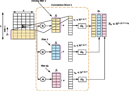
Sample convolution block. Here we illustrate how convolution operation is performed on the embedding matrix E corresponding to a given protein sequence. ‘★’ refers to the convolution operator. E is convolved with the q_k filters. Each convolution filter outputs a vector z_k that is passed through the non-linear activation function a_k, which are all combined together leading to the final feature map ${\mathbf{Z}}_{\mathbf{k}}$

2.5 Training

The DeepSol model is trained to classify protein sequences into two classes: soluble or insoluble, using a binary cross entropy objective function depicted below:

$$\text{CE}=-\sum _{n=1}^N{y}^n\ln P(y^n=1|x^n)+(1-y^n)\ln (1-P(y^n=1|x^n))$$

Here xⁿ represents the nth protein sequence and yⁿ represents its corresponding soluble or insoluble class label and N represents the total number of proteins in our training set. The models are trained for several epochs using the Adam optimizer (Kingma and Ba, 2015), which depends on various hyper-parameters such as:

• Learning rate: the step size that the optimizer should take in the parameter space while updating the model parameters.

• Batch size: the number of training examples to consider before updating the parameters.

• Maximum epochs: the total number of iterations over the training set.

• Early stopping patience: the number of epochs to wait before stopping the model training, given the validation loss does not improve.

We preset learning rate to 0.01, maximum number of epochs to 50, early stopping patience to 10 and the optimal value of the batch size tuned on the cross-validation set is found to be 64.

2.6 Evaluation metrics

The performance of DeepSol was comprehensively compared with several bioinformatics tools using evaluation metrics such as prediction accuracy and MCC. We evaluated additional quality metrics like sensitivity, selectivity and gain for each class as described in (Rawi et al., 2017).

3 Results

3.1 Hyper-parameter tuning

Our deep learning models (DeepSol S1, DeepSol S2 and DeepSol S3) for solubility prediction consisted of multiple hyper-parameters. To tune the hyper-parameters, we performed stratified 10-fold cross-validation. The hyper-parameters were tuned using a grid search procedure. The parameters and the range of values tested were as follows:

• Sequence length: The length of all protein sequences in the training, validation and test set was fixed to L = 1200, which is the length of the longest protein sequence in the dataset. Smaller than 1200 sequences were padded with zeros.

• Embedding dimensione: We tested the following settings $e\in \{50,64,100\}$⁠. We found e = 50 to be the optimal value after tuning on the validation sets, which gives us the embedding matrix, $E\in {ℝ}^{1200\times 50}$⁠.

• Convolution filter settings: For DeepSol S1, we tested three settings, given by the set of triplets $(f_k,q_k,a_k)$ (see Section 2 for explanation of notation). We drop a_k because it is fixed to ReLU for each triplet; 1) $A=\{(3,64),(7,64),(11,128)\}$⁠, 2) $B=\{(3,64),(5,64),(7,64),(11,128),(13,128),(15,128)\}$ and 3) $C=\{(2,64),(3,64),\dots ,(15,128)\}$⁠. Filter sizes (⁠$f_k\in \{2,3,\dots ,15\}$⁠) are used to extract local contexts from the protein sequence given the window size. This corresponds to the notion of a ‘biological word’ (Asgari and Mofrad, 2015) i.e. combination of amino acid residues or an amino acid k-mer. For smaller filter sizes (⁠$f_k\le 10$⁠), we used q_k = 64 while for larger filters (f_k > 10), we used q_k = 128.

  Subsequent to the multi-convolution layer, we performed global max pooling to select the maximum value from each feature map. Max pooling resulted in q_k values, each produced from a distinct convolution filter. We concatenated the values obtained after max pooling to form a compact vector representation, h. In the case of setting A, ${\mathbf{h}}_{\text{new}}=\mathbf{h}$ and ${\mathbf{h}}_{\text{new}}\in {ℝ}^{d\prime }$⁠, where $d\prime =256$⁠. The dimension of ${\mathbf{h}}_{\text{new}}$ i.e. $d\prime$ can be calculated using the formula, $d\prime ={\sum }_{k=1}^K{q}_k+\left|\mathbf{b}\right|$⁠, where $\mathbf{b}=\left\{\right\}$ for DeepSol S1, $\mathbf{b}\in {ℝ}^{57}$ for DeepSol S2 and ${\mathbf{b}}_p\in {ℝ}^p$ for DeepSol S3.

• Fully connected layer dimension (f_c): After the multi-convolution- layer gave us a vector representation ${\mathbf{h}}_{\text{new}}$⁠, we passed it through a final fully connected feed-forward layer comprising f_c neurons/units. In our experiments, the values of f_c tested were, ${\mathbf{f}}_{\mathrm{c}}\in \{64,128,256\}$⁠.

The mean performance of DeepSol models for different settings on the cross-validation sets are shown in Supplementary Figure S1. The settings B and C performed better than A and smaller value of f_c was preferred over larger values. The best performing setting was C.

Next for DeepSol S2 and DeepSol S3, we added biological features to the feature representation h that the multi-convolution-pooling layer constructed. In the DeepSol S2 setup, we concatenated the biological features directly, while for DeepSol S3, we passed biological features through a single layer feed-forward neural network. The hidden dimension of the neural network was tuned on the validation set and the optimal value was found to be 64. For testing the performance of DeepSol S2 and DeepSol S3, we primarily tested with settings B and C. A comprehensive comparison of the three DeepSol models is provided in Supplementary Table S1.

The best setting for DeepSol S2 was found to be B and the optimal value of f_c is 64. Similarly, the best setting for DeepSol S3 was C and the optimal hidden dimension for the feed-forward neural network to transform the biological features is p = 256. The best value of f_c for DeepSol S3 was 64.

The final fully connected layer for all DeepSol models (f_c) was connected to the output layer, which had two neurons, each corresponding to a class. We dropped 20% of the weights connecting any two layers in each architecture to avoid over-fitting. Each model was run for a maximum of 20 epochs with an early stopping criterion that if no improvement was observed in validation accuracy for 10 consecutive epochs, then the model building procedure would be stopped to prevent over-fitting.

Additional architectures were built (other than DeepSol S1, S2 and S3) using multi-layered and -filtered convolutional features, but their predictive performance was inferior to a model with a single layer of multi-filtered convolutional features. Detailed analysis of these models is provided in the Supplementary Material.

3.2 DeepSol performance

The prediction performance of DeepSol was assessed using an independent test set reported by (Chang et al., 2014). We compared DeepSol with solubility predictors PaRSnIP, PROSO II, CCSOL, SOLpro, PROSO, RPSP and SCM. A comprehensive comparison of DeepSol models with the best available sequence-based protein solubility predictor, PaRSnIP, and second-best predictor, PROSO II, is showcased in Figure 3.

Fig. 3.

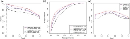
Comparison of proposed DeepSol models with PaRSnIP and PROSO II on independent test set. DeepSol S1, S2 and S3 correspond to the best DeepSol model for model Setting 1 (S1), model Setting 2 (S2) and model Setting 3 (S3), respectively. Comparison was performed with respect to area under precision-recall curve (AUPR) (Fig. 3a) and area under receiver operating curve (AUC) (Fig. 3b). We illustrate how accuracy varies as a function of the cutoff which acts as a threshold to discriminate between the soluble and the insoluble class for all these bioinformatics tools (Fig. 3c)

DeepSol S2 and S3 outperformed state-of-the-art methods like PaRSnIP and PROSO II with respect to several quality metrics, such as accuracy, selectivity and sensitivity. On the other hand, the performance of DeepSol S1, which just used CNN based features and no additional biological features, was comparable to PaRSnIP and better than PROSO II but worse than DeepSol S2 and DeepSol S3 (see Fig. 3 and Table 2). DeepSol S2 emerged as the best solubility predictor for 5 evaluation metrics yielding a prediction accuracy of 0.77 which was 3.5% better than PaRSnIP (0.74) and 19% better than PROSOII (0.64). DeepSol S2 achieved an MCC value of 0.55 which was 15% better than that obtained by either PaRSnIP (0.48) or PROSO II (0.34) (see Fig. 3a and b, and Table 2).

Table 2.

Prediction performance of DeepSol compared with seven protein solubility predictors on the independent test set

Methods	Accuracy	MCC	Selectivity (soluble)	Selectivity (insoluble)	Sensitivity (soluble)	Sensitivity (insoluble)	Gain (soluble)	Gain (insoluble)
DeepSol S1	0.73	0.46	0.75	0.71	0.69	0.77	1.50	1.42
DeepSol S2	0.77	0.55	0.84	0.72	0.65	0.88	1.69	1.44
DeepSol S3	0.77	0.54	0.81	0.73	0.69	0.84	1.63	1.46
PaRSnIP	0.74	0.48	0.76	0.72	0.70	0.78	1.52	1.45
PROSO II	0.64	0.34	0.67	0.68	0.69	0.66	1.33	1.35
CCSOL	0.54	0.08	0.54	0.54	0.51	0.57	1.09	1.08
SOLpro	0.60	0.20	0.62	0.58	0.51	0.69	1.24	1.17
PROSO	0.58	0.16	0.58	0.57	0.54	0.62	1.17	1.15
RPSP	0.52	0.03	0.52	0.51	0.44	0.59	1.03	1.02
SCM	0.60	0.21	0.65	0.57	0.42	0.77	1.30	1.14

Note: Best performing method in bold. Performance values for majority of predictors obtained from (Chang et al., 2014). Here DeepSol S1, S2 and S3 correspond to best DeepSol model for first, second and third model settings.

DeepSol S2 attained a much higher performance with respect to selectivity for soluble (0.84) and sensitivity for insoluble (0.88) proteins with respect to PaRSnIP (0.76 and 0.78 respectively). However, DeepSol S3 performed the best with respect to selectivity for soluble (0.73) and gain for insoluble (1.46) proteins. The only metric for which PaRSnIP outperformed DeepSol S2 models was on sensitivity for soluble (0.70) proteins where DeepSol S3 (0.69) was competitive with PaRSnIP. Finally, we assessed the performance of DeepSol models using different probability cutoffs (see Fig. 3c). The best performance for all bioinformatics tools (except 0.6 for PROSO II) was achieved using a threshold of 0.5, which was expected, as the training and the test sets were fairly balanced (see Table 2). We perfomed an additional comparison highlighting the superiority of the three DeepSol models over PROSO II using 10-fold cross-validation on the training set (see Supplementary Table S5). Moreover, we used 10-fold cross-validation on the training set to illustrate the stability of the results obtained by the DeepSol models for various evaluation metrics (see Supplementary Fig. S2). This is justified by the small amount of variance in the boxplots corresponding to various evaluation metrics for the different DeepSol models (see Supplementary Fig. S2).

Additionally, we built a deep feed-forward neural network classifier based on the exact set of features used in PaRSnIP. We optimized for the number of layers, the number of hidden neurons in each layer and the amount of dropout at each layer for good generalization performance and reduced the risk of over-fitting by performing 10-fold cross-validation. The optimal model, hereby referred as DL WPF (Deep Learning With PaRSnIP Features), has three feed-forward layers with 128 hidden neurons each and a dropout of 20%. We could not use CNNs as the local contextual features (mono-, di- and tri-peptide frequencies) from the raw protein sequences were engineered explicitly for PaRSnIP. DL WPF achieved an accuracy of 0.70 and a MCC value of 0.39 on the independent test set. For DL WPF both accuracy and MCC values were much smaller in comparison to that obtained from PaRSnIP and DeepSol S2 indicating a feed-forward neural network built on PaRSnIP features was not as capable as either PaRSnIP (GBM) or DeepSol S2 (CNN) for protein solubility prediction.

By using score distribution plots, we were able to compare DL WPF with PaRSnIP and the best proposed approach, DeepSol S2, to identify whether the improvement came from the training algorithm or from the selection of features (see Fig. 4a). It empirically illustrated that the score distributions for the three methods did not follow a normal distribution. Hence, we used the Mann-Whitney-Wilcox (MWW) test (Mann and Whitney, 1947) to compare pairwise score distribution for each class. We found that the score distributions of DeepSol S2 versus DL WPF, DL WPF versus PaRSnIP and DeepSol S2 versus PaRSnIP were all different (P-value < 0.01) in the case of the insoluble class and the difference between the mean scores for each of the paired score distributions (DeepSol S2 versus DL WPF and DL WPF versus PaRSnIP) were statistically significant (P-value < 0.01) for the soluble class. Moreover, from the violin plot, we observed that the score distributions followed very different density distributions for the three methods, particularly in the case of the insoluble class (see Fig. 4a). This indicated that the underlying mechanism being used by these models for classifying the insoluble class prediction was disparate. Both DL WPF and PaRSnIP used the same set of features, but PaRSnIP built more accurate gradient boosted trees, resulting in a score distribution that contrasted with the one obtained from DL WPF for both the soluble and the insoluble class. Additionally, at the optimal cutoff 0.5, DL WPF had greater density of scores below threshold θ for the soluble class, resulting in lower accuracy than DeepSol S2 and PaRSnIP.

Fig. 4.

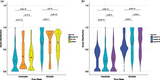
Comparison of score distributions for various protein solubility predictors. PaRSnIP and DeepSol S2 have nearly similar score distributions (no statistical significance) for the soluble class but these are very different for the insoluble class. However, in Figure 4b, only DeepSol S2 and DeepSol S3 have similar shapes for score distributions in the cases of both the soluble and the insoluble class. The violin plot corresponding to each method for each class can efficiently estimate the density of the scores, with thickness $\propto$ to the density. Here the ‘dark red’ colored diamond represents the mean for each score distribution, P represents P-value and 2e-16 is equivalent to $2\times {10}^{-16}$⁠. (a) Comparison of score distributions of DeepSol S2, DL WPF and PaRSnIP for both insoluble and soluble test set proteins. (b) Comparison of score distributions of DeepSol S1, S2 and S3 for both insoluble and soluble test set proteins

Interestingly, DeepSol S2 was the only method that was >99% confident while predicting both the soluble (score = 1) and the insoluble (score = 0) class for several test set proteins (see Fig. 4a). Another interesting observation was that DeepSol S2 and PaRSnIP had a similar score distribution for the soluble class (P-value $=$ 0.74) and the mean score for DeepSol S2 (0.24) was significantly lower than the mean score for PaRSnIP (0.32) in case of the insoluble class. Lower score values are better for the insoluble class where the actual class label is 0 and higher score values are better for soluble class where the actual class label is 1.

Similarly, we showed empirically that score distributions for the three DeepSol model settings did not follow the normal distribution (see Fig. 4b). Hence, we performed the MWW test between pairwise distributions (DeepSol S1 versus DeepSol S2, DeepSol S2 versus DeepSol S3, DeepSol S3 versus DeepSol S1) for both the insoluble and the soluble class, respectively. The difference between the mean scores for each paired score distribution was statistically significant for both the insoluble and the soluble class. At the optimal prediction cutoff 0.5, DeepSol S1 had a higher density of scores ≥0.5 for the insoluble class and a higher density of scores ≤0.5 for the soluble proteins, resulting in lower predictive accuracy and MCC in comparison to DeepSol S2 and DeepSol S3. Moreover, from the violin plot, we observed that the score density distribution of DeepSol S1 was very different from that of DeepSol S2 and DeepSol S3 in the case of both the insoluble and the soluble class (see Fig. 4a). Though the underlying mechanism being used by all DeepSol models was CNN based Deep Learning, DeepSol S2 and DeepSol S3 benefit similarly from the additional 57 biological features resulting in more accurate models (having almost identical density distributions for both the classes) in comparison to DeepSol S1 (see Table 2).

4 Discussion

Novel in silico, sequence-based protein solubility predictors that have high prediction accuracy are highly sought. In this study, we introduce DeepSol, a solubility predictor that uses Deep Learning, in particular CNNs, and additional set of biological features that represent sequence as well as structural properties of proteins. DeepSol (S2 and S3) outperformed, to the best of our knowledge, all existing sequence-based solubility predictors by at least 3.5% in accuracy and 15% in MCC.

Interestingly, the performance of DeepSol S1, which extracts local contextual feature vectors using ‘biological’ words of different lengths (⁠$f_k\in \{2,3,\dots ,15\}$⁠) from just the raw protein sequence, is comparable with PaRSnIP and much better than SVM-based tools like PROSO II, CCSOL and SOLpro with respect to various evaluation metrics. PaRSnIP uses 8477 features including mono-, di- and tri-peptide frequencies along with an additional 57 biological features mentioned in Table 1. The authors of PaRSnIP illustrated that k-mer peptide frequencies (where $k\in \{1,2,3\}$⁠) play a major role in predicting the solubility of a protein. However, this suggests that DeepSol S1 not only captures mono-, di- and tri-peptide frequencies through the local contextual feature vector, but can also capture additional informative higher order interactions amidst the amino acid residues by means of the convolutional features (⁠$f_k\in \{4,5,\dots ,15\}$⁠) and higher order abstract structural features such as protein folds (Hou et al., 2017), thereby, making its predictive performance comparable to PaRSnIP (see Table 2). It was shown in (Hou et al., 2017) that CNNs can be used to accurately predict protein folds and in a recent review on protein solubility (Trainor et al., 2017), the authors emphasize that sequence-based features such as k-mer frequencies and structural features such as protein folding play a vital role in protein solubility.

One of the limitations of PaRSnIP is that it explicitly calculates the peptide frequency for different values of k. Hence, for larger values of k, the computational complexity explodes (i.e. ${20}^k$ features), whereas CNNs can capture these higher order local interactions with relative ease using multiple parallel non-linear convolution filters. However, PaRSnIP has the ability to provide relative variable importance for each feature, a trait currently missing in the DeepSol architecture.

DeepSol S2 and S3 models have score means which are closer to each other for both soluble and insoluble classes in comparison to DeepSol S1 (see Fig. 4b). This is expected as they both greatly benefit from complimentary information incorporated in these models through the additional 57 explicit sequence and structural features. Both, DeepSol S2 and DeepSol S3 achieve superior performance for each class (see Table 2 and Fig. 4b). This indicated that local contextual feature vectors learnt via a multi-filter CNN is complimented by sequence and structural features such as FERs, SS features obtained from SCRATCH, hydrophobicity indices of exposed residues, etc. and are not confounding each other. It was shown in PaRSnIP (Rawi et al., 2017) that several of these additional explicit features also play a major role in protein solubility prediction. Moreover, as in DeepSol S1, both DeepSol S2 and DeepSol S3 capture discriminative higher order local interactions amidst the amino acid residues by means of the different convolution filter sizes (⁠$f_k\in \{4,5,\dots ,15\}$⁠), thereby, making its predictive performance superior.

Finally, the primary reason for the enhanced performance of DeepSol models is the choice of state-of-the-art machine learning technique CNNs. The CNN framework exploits the k-mer structure in the input protein sequence using a set of parallel convolution filters of varying sizes and can efficiently capture abstract structural features such as protein folds (Hou et al., 2017). It can inherently capture the non-linear relationships between the local contextual feature vector and the dependent vector (solubility classification), while preventing over-fitting using dropout on the weights, leading to good generalization performance. It overcomes the limitations faced by two-stage classifiers which have a separate step for feature selection. Moreover, the predictive performance of DeepSol models (DeepSol S2 and S3) is significantly boosted by the addition of 57 sequence and structural features extracted from protein sequences using bioinformatics tools (e.g. SCRATCH) which compliment the local contextual feature vector obtained from multi-filter CNN.

In conclusion, we propose a novel Deep Learning-based solubility predictor, DeepSol, that primarily utilizes features extracted from the raw protein sequence using CNNs. The performance of DeepSol is boosted by additional sequence and structural features extracted from the protein sequence. DeepSol overcomes limitations such as two-stage classifier with a separate step for feature selection and outperforms all existing sequence-based solubility predictors with respect to various evaluation metrics like accuracy, MCC, selectivity and gain for soluble and sensitivity for insoluble proteins.

The capability (sensitivity) of DeepSol S1 (69%) and DeepSol S3 (69%) to correctly identify soluble proteins in the independent test set is comparable to that of sequence-based methods like PaRSnIP (70%) and PROSO II (69%). However, DeepSol S2 (88%) and DeepSol S3 (84%) are 10 and 6% more sensitive than PaRSnIP (78%), respectively, and are 22 and 18% more sensitive than PROSO II (66%), respectively for identifying insoluble proteins. Hence, DeepSol can be applied in applications, such as, to pre-reject initial targets that are insoluble in silico and thus can help to reduce the production cost.

Conflict of Interest: none declared.