ddPCRclust: an R package and Shiny app for automated analysis of multiplexed ddPCR data

Abstract

Motivation

Droplet digital PCR (ddPCR) is an emerging technology for quantifying DNA. By partitioning the target DNA into ∼20 000 droplets, each serving as its own PCR reaction compartment, a very high sensitivity of DNA quantification can be achieved. However, manual analysis of the data is time consuming and algorithms for automated analysis of non-orthogonal, multiplexed ddPCR data are unavailable, presenting a major bottleneck for the advancement of ddPCR transitioning from low-throughput to high-throughput.

Results

ddPCRclust is an R package for automated analysis of data from Bio-Rad’s droplet digital PCR systems (QX100 and QX200). It can automatically analyze and visualize multiplexed ddPCR experiments with up to four targets per reaction. Results are on par with manual analysis, but only take minutes to compute instead of hours. The accompanying Shiny app ddPCRvis provides easy access to the functionalities of ddPCRclust through a web-browser based GUI.

Availability and implementation

R package: https://github.com/bgbrink/ddPCRclust; Interface: https://github.com/bgbrink/ddPCRvis/; Web: https://bibiserv.cebitec.uni-bielefeld.de/ddPCRvis/.

Supplementary information

Supplementary data are available at Bioinformatics online.

1 Introduction

Droplet digital PCR (ddPCR) is an emerging technology for detection and quantification of nucleic acids. In contrast to other digital PCR approaches, it utilizes a water-oil emulsion droplet system to partition the template DNA molecules. Each one of typically around 20 000 nanoliter-sized droplets serves as a compartment for a PCR reaction. The PCR reaction is carried out until its plateau phase, eliminating amplification efficiency bias. Each genetic target is fluorescently labelled with a combination of two fluorophores (typically HEX and FAM), giving it a unique footprint in a two-dimensional space represented by the intensities per colour channel. The position of each droplet within this space reveals how many and, more importantly, which genetic targets it contains. Thus, droplets that contain the same combination of targets, cluster together. The number of positive droplets for each target determines its abundance, which can for instance be used to detect copy number aberrations in clinical samples.

However, in clinical formalin-fixed paraffin-embedded (FFPE) samples, damage in the form of sequence alterations can further reduce the amplification efficiency, in addition to the low quantity and quality of the DNA generally obtained. This results in droplets with their respective signal lying along a vector connecting two clusters in the ddPCR output, which is commonly called rain (Jones et al., 2014). A recently published protocol by Hughesman et al. (2016) describes a protocol for multiplexing (i.e. using reactions with more than two targets) ddPCR with clinical FFPE samples by using a combination of flourophores to obtain a non-orthogonal layout in order to avoid overlapping rain (see Fig. 1b).

Fig. 1.

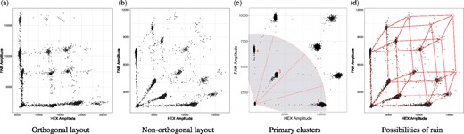
During a ddPCR run, each genetic target is fluorescently labelled with a combination of two fluorophores. The position of each droplet within this space reveals how many and, more importantly, which genetic targets it contains. Thus, droplets that contain the same targets, or the same combination of targets, cluster together. In clinical FFPE samples, DNA might be partially degraded, causing formation of rain and disappearance of the higher order clusters. (a) Multiplexing can cause overlap of clusters and rain. (b) Non-orthogonal layout avoids overlap of clusters and rain. (c) The angles between the droplets on the bottom left, which retain no target, and the primary clusters are highlighted. In case of genomic deletions or purposely missing clusters, it is possible to determine which cluster is missing. In this case, a genetic deletion of target 2 has occurred. (d) Graphical representation of the possible formation of rain along vectors

Several automated methods have been developed (Attali et al., 2016; Chiu et al., 2017; Dobnik et al., 2016; Jacobs et al., 2017; Trypsteen et al., 2015) to analyze ddPCR data. However, analysis of non-orthogonal, multiplexed ddPCR reactions is not supported by any tool. To overcome these limitations, we developed the ddPCRclust algorithm, an R package and associated interface (ddPCRvis) for automated analysis of multiplexed ddPCR samples.

2 Materials and methods

As aforementioned, data from ddPCR consists of a number of different clusters l₁,…, l_k and their respective centroids c₁,…, c_k, where k is the number of clusters. All droplets (x₁,…, x_m) represent one or more genetic targets t₁,…, t_n, where m is the number of droplets and n is the number of targets. Each cluster l_i is defined as a group of droplets that contain an identical combination of targets. We define four steps to successfully analyze this data, each step is detailed in subsection 2.2.

1. Find all cluster centroids c.

2. Assign one or multiple targets t to each cluster l based on c.

3. Allocate the rain and assign a cluster label l to each droplet x.

4. Determine the number of positive droplets for each target t and calculate the CPDs.

The algorithm was implemented in R (R Core Team, 2017) and can be installed as a package. The main function of the package is ddPCRclust. This function runs the algorithm with one or multiple files. Automatic distribution among all CPU cores is optional (not supported on Windows).

2.1 Input data

The input data are one or multiple CSV files containing the raw data from Bio-Rad’s droplet digital PCR systems (QX100 and QX200). Each file can be represented as a two-dimensional data frame. Each row within the data frame represents a single droplet, each column the respective intensities per colour channel.

2.2 Clustering

Step 1—Cluster centroids: We find the centroids of the clusters based on three different approaches; flowDensity (Malek et al., 2015), SamSPECTRAL (Zare et al., 2010) and flowPeaks (Ge and Sealfon, 2012). We adjusted parameters of each algorithm to provide the best results on ddPCR data. Each approach has its own function within ddPCRclust, provided users need more granular control. To label clusters we start with the bottom left cluster, which is assigned to the population of empty droplets, i.e. the droplets showing no signal for any of the targets.

Step 2—Cluster labelling: The clusters with the droplets that contain only a single target form a sector with the population of empty droplets (see Fig. 1c). We use the angle between the population of empty droplets and the respective first order clusters to label them correctly. We then estimate the position of higher order clusters based on the location of the first order clusters. To do so, we create a distance matrix, containing the distances between the estimated cluster positions and all cluster centres found by the algorithms. The optimal assignment for each cluster can then be calculated by solving the Linear Sum Assignment Problem using the Hungarian Method (Papadimitriou and Steiglitz, 1982).

Step 3—Rain allocation: Certain ddPCR experiments can involve rain, which can contain up to half of the droplets intrinsically belonging to the higher order cluster. Thus, accurate allocation of rain is a crucial part of the algorithm. To do so, we have to find the minimal distance between each droplet and each cluster, as well as between each droplet and the respective vectors connecting the clusters (see Fig. 1d). However, an all-vs-all comparison has a significant impact on the runtime of the algorithm $(\mathcal{O}(2^{n-1}(n+2)m))$⁠. This number can be reduced by preprocessing the data. Filtering out points that are obviously not rain, can greatly demagnify n, speeding up the algorithm significantly in the process. The obvious choices are points that are sufficiently close to the cluster centres. To estimate the distance of a point to a cluster centre, we use an empirically derived Mahalanobis distance threshold (Mahalanobis, 1936). Furthermore, only taking clusters and vectors in the vicinity of the droplet into account will lower the number of operations even further. The whole function is comprised of the following steps:

1. For each cluster centre c, calculate the Mahalanobis distance d_M to each point based on the covariance matrix of the dataset.

2. Remove all points where d_M < mean(d_M) for the respective cluster. Those points are closer than the average around the respective cluster centres and hence do not have to be considered as rain.

3. For each cluster centre c, remove all points that are not in between c and the respective higher order clusters.

4. For all remaining points, perform the all-vs-all comparison as described earlier.

The intermediary result is three arrays of unique identifiers, which represent the cluster membership for each row of the data frame. Each array is the result from one of the three independent clustering approaches. Next, these results need to be combined.

Step 4—CPDs calculation: Until this point, all three approaches were computed independently. To compute the final result, we create a cluster ensemble using the clue package for R (Hornik, 2005). The results of the previous clusterings are first converted into partitions before the medoid of the cluster ensemble is computed. As a measure of confidence, the agreement of the cluster ensemble is calculated using the adjusted Rand index (Hubert and Arabie, 1985).

Once all droplets are correctly assigned, the copies per droplet (CPDs) for each target are calculated by the function calculateCPDs. In order to compare individual wells (or files) with each other, a constant reference control is required. This target should be a genetic region that is usually not affected by any variations and is present in every file. If the name of this marker is provided, all CPDs will be normalized against it.

2.3 Exporting results

The results can be exported using exportPlots, exportToExcel and exportToCSV.

2.4 ddPCRvis

ddPCRvis is a GUI that gives access to the aforementioned functionalities of the ddPCRclust package directly through a web browser, powered by R Shiny (Chang et al., 2017). It also enables the user to check the results and manually correct them if necessary.

3 Results

Along with the algorithm, we provide a set of eight representative example files. We compared the clustering results of ddPCRclust to manual analysis by experts using the adjusted Rand index. The results for those eight reactions are presented in Table 1.

Table 1.

Run time and accuracy compared to manual annotation by experts for eight exemplary reactions provided alongside the R package

Total number of droplets	Adjusted Rand index	Run time in seconds
14590 (1295)	0.997 (0.003)	7.18 (1.98)

Note: Computed on Intel(R) Core(TM) i7-4650U CPU @ 1.70GHz and 8 GB RAM. Each entry comprises the mean and the standard deviation, the latter being in brackets.

4 Discussion

While the advantages of digital PCR in terms of sensitivity and accuracy have already been established, the technology has long been held back by its low throughput compared to other techniques. The advancement of using thousands of nanoliter droplets instead of physical wells paired with new protocols for multiplexed ddPCR reactions will provide a boost to the field of digital PCR. These new types of data require new computational methods to be devised in order to aid the technology on the analysis end. Automated analysis of non-orthogonal reactions was not yet possible and manual analysis takes many hours to complete, while suffering the usual disadvantages of subjectivity and non-reproducibility.

We developed ddPCRclust, an R package which can automatically calculate CPDs for multiplexed ddPCR reactions with up to four targets in a non-orthogonal layout. Results of ddPCRclust are on par with manual annotation by experts, while the computation only takes a few minutes per 96-well experiment. As with every clustering method, it is impossible to achieve perfect accuracy and low DNA concentration, which causes very sparse clusters, still provides a challenge (see Supplementary Fig. S1). Thus, we implemented three independent clustering approaches to provide more robustness, which is especially important in a medical context. Furthermore, the underlying distribution of the clusters could be subject to further studies.

A visual interface is crucial for users to have a mental model of their data and easy accessibility without having to download and install the R package, in turn saving time and effort. ddPCRvis based on the Shiny package provides that and also enables the user to check the results and manually correct them if necessary.

Acknowledgements

We like to thank X. J. David Lu and Dr. Curtis B. Hughesman for their invaluable contributions in designing multiplexed ddPCRs, preparing data and testing the software. We further like to thank Dr. Charles Haynes, Dr. Catherine Poh and Dr.-Ing. Tim W. Nattkemper for their continuous support throughout the project.

Funding

This work was funded by the International DFG Research Training Group GRK 1906/1 and by NSERC.

Conflict of Interest: none declared.