Hierarchical HotNet: identifying hierarchies of altered subnetworks

Abstract

Motivation

The analysis of high-dimensional ‘omics data is often informed by the use of biological interaction networks. For example, protein–protein interaction networks have been used to analyze gene expression data, to prioritize germline variants, and to identify somatic driver mutations in cancer. In these and other applications, the underlying computational problem is to identify altered subnetworks containing genes that are both highly altered in an ‘omics dataset and are topologically close (e.g. connected) on an interaction network.

Results

We introduce Hierarchical HotNet, an algorithm that finds a hierarchy of altered subnetworks. Hierarchical HotNet assesses the statistical significance of the resulting subnetworks over a range of biological scales and explicitly controls for ascertainment bias in the network. We evaluate the performance of Hierarchical HotNet and several other algorithms that identify altered subnetworks on the problem of predicting cancer genes and significantly mutated subnetworks. On somatic mutation data from The Cancer Genome Atlas, Hierarchical HotNet outperforms other methods and identifies significantly mutated subnetworks containing both well-known cancer genes and candidate cancer genes that are rarely mutated in the cohort. Hierarchical HotNet is a robust algorithm for identifying altered subnetworks across different ‘omics datasets.

Availability and implementation

http://github.com/raphael-group/hierarchical-hotnet.

Supplementary information

Supplementary material are available at Bioinformatics online.

1 Introduction

Many cellular processes involve interactions between different molecules. Therefore, the analysis and interpretation of large-scale ‘omics data is often informed by biological interaction networks. For example, the expression of genes in the same protein complex or pathway is often correlated (Ge et al., 2001), so physical interaction networks can be used to study gene expression data (Luscombe et al., 2004). Similarly, genetic variants associated with a disease often cluster in a small number of biological processes, and therefore networks can be used to analyze germline variants from genome-wide association studies (GWAS) (Califano et al., 2012; Lee et al., 2011; Leiserson et al., 2013) or somatic mutations in cancer (Leiserson et al., 2015; Vandin et al., 2011). In these applications, one has a measurement, or score, on each of the vertices in a network, and the goal is to identify altered subnetworks, or sets of vertices that are both close on the network and have high scores.

A specific example of the general problem of identifying altered subnetworks arises in cancer genomics. In this case, one obtains measurements of somatic mutations from a cohort of cancer patients and aims to distinguish the small number of driver mutations that are typically responsible for tumor initiation and development from the much larger number of random passenger mutations. Tests for recurrence of individual mutations or genes (Kandoth et al., 2013; Lawrence et al., 2013; Mularoni et al., 2016) are often challenged by the ‘long tail’ phenomenon, where most driver mutations are extremely rare in the cohort. By taking advantage of the observation that driver mutations tend to cluster in a few key biological processes (e.g. cell cycle or apoptosis) (Hanahan and Weinberg, 2011; Vogelstein et al., 2013), one can use protein–protein interaction (PPI) networks to identify significantly mutated sets of interacting genes (Cowen et al., 2017; Raphael et al., 2014). These gene sets may span multiple biological scales, from interacting gene pairs through protein complexes and pathways to entire biological systems (Fig. 1). Hierarchies are commonly used to describe relationships between gene sets across different scales; gene ontologies (GO) (Ashburner et al., 2000) are one such example.

Fig. 1.

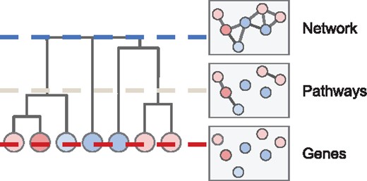
Illustration of a hierarchy of gene sets, which vary in size across different biological scales

A number of methods have been developed to address the problem of identifying altered subnetworks. We broadly classify these methods into three groups. The first group of methods defines a restricted class of candidate subnetworks and then select high-weight subnetworks from these candidates according to their vertex scores. Examples of these methods include jActiveModules (Ideker et al., 2002) and heinz/BioNet (Beisser et al., 2010; Dittrich et al., 2008) which solve the maximum-weight connected subgraph (MWCS) problem. Other methods, such as MUFFINN (Cho et al., 2016) and NetSig (Horn et al., 2018) examine only the nearest neighbors of each vertex, thus assigning a score to ‘star subnetworks’ centered on every vertex. A related approach is used in Omics Integrator (Tuncbag et al., 2013, 2016), which solves a variation of the prize-collecting Steiner forest (PCSF) problem.

The second group of computational methods search for high-weight subnetworks by jointly examining vertex scores and network topology. These methods are able to identify subnetworks that would not be considered using vertex scores or topology alone. Many such methods use a diffusion process or random walk to measure the similarity of pairs of nodes using the paths between them (Cowen et al., 2017). Heat diffusion and random walks are common tools for biological network analysis (e.g. Cao et al., 2013; Cho et al., 2015; Chung and Zhao, 2010; Hofree et al., 2013; Komurov et al., 2012; Paull et al., 2013; Shnaps et al., 2016). PRINCE (Vanunu et al., 2010), HotNet (Vandin et al., 2011, 2012), HotNet2 (Leiserson et al., 2015) and Ruffalo et al. (2015) are examples of this group of methods.

The third group of computational methods is similar to the first and second groups, but these methods incorporate additional information, including predefined pathways [e.g. PARADIGM (Vaske et al., 2010) and DEGraph (Jacob et al., 2012)], mutual exclusivity and/or co-occurrence of mutations among genes/proteins [e.g. MEMo (Ciriello et al., 2012), MEMCover (Kim et al., 2015) and BeWith (Dao et al., 2017)], or connections between mutations and expression (e.g. Kim et al., 2011 and HIT’nDRIVE (Shrestha et al., 2017)). These methods leverage additional hypotheses and/or data in their application domains, often improving their predictions for specific applications but potentially limiting their extension to other areas.

In this article, we introduce a novel computational method, Hierarchical HotNet, to identify altered subnetworks. Hierarchical HotNet addresses several limitations with existing approaches. Key features of Hierarchical HotNet include integration of both network topology and vertex scores; robustness to new and complex datasets; combating ascertainment bias in data, e.g. recurrently mutated genes tend to be better studied with more known interactions; and evaluating the statistical significance of results. Table 1 compares features for several state-of-the-art approaches.

Table 1.

Features of several methods for identification of altered subnetworks

Feature/Method	heinz	MUFFINN	NetSig	HotNet2	Hierarchical HotNet
Candidate subnetworks	Connected subnetworks	Nearest neighbor subnetworks	Nearest neighbor subnetworks	Unrestricted	Unrestricted
Evaluates statistical significance	No	No	Yes, network permutations	Yes, multiple options	Yes, multiple options
Addresses ascertainment bias in network	No	No	Degree-aware statistical test	Penalizes high-degree nodes	Penalizes high-degree nodes; degree-aware statistical test
Model selection	Yes, on data	No	Yes, on results	No	Yes, on results
Consensus across datasets	No	No	No	Yes	Yes
Supported interaction types	Unweighted and undirected	Weighted and undirected	Unweighted and undirected	Unweighted and undirected	Weighted and directed

Hierarchical HotNet jointly considers network topology and vertex scores (i.e. it belongs to the second of the above groups of methods) to construct a hierarchy of topologically close and high-scoring subnetworks. It uses a rigorous approach to identify statistically significant subnetworks across different regions of its hierarchy, providing relationships between subnetworks. Applied to cancer genomics data, Hierarchical HotNet identifies significantly mutated subnetworks across biological scales.

We evaluate the performance of Hierarchical HotNet on the problem of finding mutated subnetworks in cancer using two recent pan-cancer somatic mutation datasets and three interaction networks. We compare Hierarchical HotNet to heinz, MUFFINN, NetSig and HotNet2 as representative methods from the above groups. Hierarchical HotNet outperforms these other methods in identifying known and candidate cancer genes. Hierarchical HotNet also prioritizes many putative cancer genes that are not statistically significant by single-gene tests.

2 Materials and methods

Given a network or graph $G=(V,E,w)$ with $n=\left|V\right|$ vertices, $m=\left|E\right|$ edges and scores/weights $w(v_1),\hspace{0.17em}\dots ,w(v_n)$ on the vertices, Hierarchical HotNet aims to hierarchically cluster high-weight vertices that are topologically close on the network and identify statistically significant subnetworks in the hierarchy. More specifically, Hierarchical HotNet (i) combines network topology and vertex scores, (ii) defines a similarity matrix S from G using a random walk-based approach as described in Section 2.1, (iii) constructs a hierarchy of clusters consisting of strongly connected components (SCCs) as described in Section 2.2, (iv) assesses the statistical significance of clusters in the hierarchy as described in Section 2.3, (v) identifies altered clusters from statistically significant regions of the hierarchy and (vi) combines these clusters from multiple networks and sets of vertex scores as described in Section 2.4. Figure 2 shows an overview of the Hierarchical HotNet method in the context of biological data.

Fig. 2.

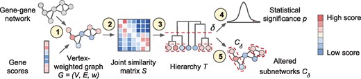
Overview of the Hierarchical HotNet method. (1) A biological interaction network and gene scores are paired to form a vertex-weighted graph $G=(V,E,w)$⁠. (2) A joint similarity matrix S is derived from both network topology and vertex weights using a random walk-based approach. (3) A dendrogram T of vertex sets is constructed from S using asymmetric hierarchical clustering. (4) The statistical significance p of T is evaluated (test statistic and null model for G not shown). (5) Representative altered subnetworks $C_{\delta }$ are provided from the dendrogram T

2.1 Similarity matrix S for vertex-weighted graph G

In order to characterize groups of related vertices in the vertex-weighted graph G, we define a similarity measure between pairs of vertices. Any such measure yields a similarity matrix $S=[s_{ij}]$⁠, where s_ij measures how similar a vertex v_j is to a vertex v_i according to both network topology and the vertex scores. By incorporating both topology and scores, this measure allows us to quantify proximity in a vertex-weighted graph beyond the topological structure of the graph or the weights on the vertices.

The network itself describes a particularly simple similarity measure that is given by the adjacency matrix of the graph, where two vertices are defined to be similar if and only if they share an edge. Beyond nearest neighbors (Eppstein et al., 1997), diffusion kernels (Kondor and Lafferty, 2002; Schölkopf et al., 2004; Vandin et al., 2011, 2012), random walks (Chung, 2007; Chung and Zhao, 2010; Leiserson et al., 2015) and other measures (Yip and Horvath, 2006) define similarity beyond the presence or absence of direct interactions. These similarity measures capture network topology or use network topology to ‘smooth’ or reprioritize the scores over the network (Ruffalo et al., 2015; Vanunu et al., 2010), resulting in network-adjusted vertex weights.

In contrast, Hierarchical HotNet defines a similarity measure using both network topology and vertex scores. HotNet (Vandin et al., 2011, 2012) uses a diffusion kernel to model heat diffusion over the edges of a graph, while HotNet2 Leiserson et al. (2015) and Hierarchical HotNet use a random walk, which is a stochastic process describing evolving distributions on the vertices of a graph. In a common version of the random walk with restart, a random walker traverses the graph in a series of discrete steps, transitioning to one of its neighbors at each step with probability β and returning to its initial position with probability $1-\beta$⁠, leading to a non-trivial stationary distribution. We use this stationary distribution to define the following similarity matrix.

We now derive the similarity matrix for a simple vertex-weighted graph. Details for directed and weighted edges are in the Supplementary Material. Let A be an adjacency matrix for a vertex-weighted graph G and let $D=\text{diag}(\mathrm{deg}(G))=\text{diag}(d_1,\dots ,d_n)$ be the corresponding diagonal degree matrix. We define a topological similarity matrix

$$P=\beta {(I-(1-\beta )A{D}^{-1})}^{-1}$$

(1)

using the stationary distribution of the random walk with restart. This matrix is a stochastic matrix whose columns are probability vectors. We scale the columns of P with the vertex weights w to define a joint similarity matrix $S=[s_{ij}]=P\times \text{diag}\left(w(v_1),\dots ,w(v_n)\right)$⁠, where

$$s_{ij}=w(v_j)\left(\beta (1-\beta )\frac{a_{ij}}{d_j}+\beta {(1-\beta )}^2{\displaystyle \sum _{k=1}^n\frac{a_{ik}}{d_k}\frac{a_{kj}}{d_j}}+\cdots \right).$$

(2)

Note that (2) explicitly addresses network ascertainment bias by penalizing high-degree vertices. Note, too, that both P and S are asymmetric, allowing these matrices to capture potentially asymmetric relationships.

See the Supplementary Material for a more detailed discussion of S, including a procedure for choosing the restart probability β that preserves the locality of the random walk with restart.

2.2 Hierarchy T for similarity matrix S

We identify subnetworks in the graph G by finding clusters using the similarity matrix S. Most clustering algorithms rely, either explicitly or implicitly, on one or more parameters and a variety of clustering algorithms, including k-means clustering, network modularity, density-based clustering and spectral clustering, give rise to parameterized families of vertex clusterings. Often, the resulting clusters are sensitive to the values of these parameters. Procedures for selecting parameter values may be sensitive to the chosen training datasets or computationally expensive and the recommended parameter values may reflect unstated assumptions about the data. Applying a clustering algorithm over all parameter values of potential interest may be computationally or statistically infeasible.

Hierarchical clustering algorithms provide parameterized families of vertex clusterings in the form of a hierarchy or dendrogram, where the height of a dendrogram corresponds to the choice of a clustering parameter. Hierarchical clustering reduces the need for clustering parameter selection, providing clusters over all possible parameter values as well as relationships between the clusters themselves.

Given a similarity matrix S, a hierarchical clustering method can produce a parameterized family ${\left\{C_{\delta }\right\}}_{\delta }$ of clusterings, where the relationships between the clusters can be described with a dendrogram T. The clustering parameter δ corresponds to a height of the dendrogram T and a cut of T at δ corresponds to a clustering, or partitioning, $C_{\delta }$ of the vertices. Since S is a similarity matrix, smaller values of δ produce larger clusters $C_{\delta }$ and larger values of produce smaller clusters. Each vertex of T is a cluster $C\subseteq V$ and the height δ of a vertex in T is the largest value of δ for which $C\in {\mathcal{\text{C}}}_{\delta }$⁠. There is a leaf vertex in T for each vertex $v\in V$ and there is a single root vertex in T for the set V. The relationships between the leaf vertices, the inner vertices and the root vertex of T produce a substructure of clusters.

Single-, average- and complete-linkage clustering are common examples of hierarchical clustering algorithms for symmetric similarity or dissimilarity matrices (see Defays, 1977; Sibson 1973). Hierarchical clustering algorithms for asymmetric matrices are less common (Malliaros and Vazirgiannis, 2013).

In particular, we perform the following hierarchical clustering procedure, which preserves asymmetric relationships between genes. For $\delta \ge 0$⁠, let $H_{\delta }=(V,E_{\delta })$ be a directed graph with $E_{\delta }=\{(v_j,v_i)\in V\times V:s_{ij}\ge \delta \}$ and let $C_{\delta }$ be the SCCs of $H_{\delta }$⁠. This parameterized family ${\left\{C_{\delta }\right\}}_{\delta }$ induces a dendrogram T, where smaller values of δ correspond to larger clusters $C_{\delta }$ higher in T.Hubert (1973) first discussed using SCCs for hierarchical clustering with asymmetric similarity matrices, which is equivalent to single linkage clustering when S is symmetric. Tarjan (1983) described an $O(n^2\log n)$-time algorithm for this procedure, which we used for Hierarchical HotNet. To the authors’ knowledge, hierarchical clustering with SCCs has not been widely used; see Slater (1984) for one example.

2.3 Statistical significance for hierarchy T

Given a dendrogram T describing a parameterized family ${\left\{C_{\delta }\right\}}_{\delta }$ of vertex clusters for a vertex-weighted graph G, we want to evaluate whether there are clusters in T (corresponding to altered subnetworks in G) whose vertices have higher scores/weights than expected by chance. For such a test, we require a null hypothesis and a test statistic. A natural and commonly used null hypothesis is that the vertex weights are independent of network topology. However, this is not a well-formed null hypothesis as the notion of independence needs to be defined more precisely. We describe three null distributions that preserve different features of the vertex weights and/or network topology.

2.3.1 Random vertex-weighted graphs

Graphs with prescribed vertex weights

We define an ensemble of vertex-weighted graphs with the same vertices and edges as the observed graph G. Formally, we define

$${\mathcal{G}}_w=\left\{G\prime =(V,E,w\prime ):w\prime =\pi (w)\text{ for }\pi \in \Pi \right\},$$

(3)

where Π is the collection of all permutations of vertex weights.

We consider the uniform distribution on ${\mathcal{G}}_w$⁠, and we sample uniformly from ${\mathcal{G}}_w$ by permuting the assignment of weights to vertices. Note that HotNet2 uses this permutation scheme as part of its statistical test.

Graphs with prescribed vertex weights correlated with degree

In many biological applications, vertex weights are correlated with vertex degree. This is often due to ascertainment bias, as high-scoring genes are frequently better studied and thus more of their interactions tend to be known and represented in networks. We define an ensemble of vertex-weighted graphs to preserve a correlation between vertex weights and degree. To preserve the exact correlation between the observed vertex weights and vertex degree, one might permute weights only among vertices with the same degree. However, in most biological networks, most degrees are unique or shared by few nodes. Thus, we partition vertices into bins according to their degree and preserve the vertex weights within each bin to define an ensemble ${\mathcal{G}}_w^{\ell }\subseteq {\mathcal{G}}_w$⁠. In particular, we partition V into bins V₁, …, V_k such that (i) vertices with the same degree belong to the same bin, i.e. if $\mathrm{deg}(u)=\mathrm{deg}(v)$⁠, then $u,v\in V_i$ for some i; (ii) each bin has at least $\ell$ vertices; and (iii) the following quantity is minimized:

$$\underset{\left|V_1\right|,\dots ,\left|V_k\right|\ge \ell }{\min }{\displaystyle \sum _{i=1}^k\left(\underset{v\in V_i}{\max }\mathrm{deg}(v)-\underset{v\in V_i}{\min }\mathrm{deg}(v)\right)}.$$

(4)

This partition minimizes the differences in vertex degrees within bins while enforcing a minimum number $\ell$ of permuted vertex weights within each bin. Formally, we define

$${\mathcal{G}}_w^{\ell }=\left\{G\prime =(V,E,w\prime ):w\prime =\pi (w)\text{ for }\pi \in {\Pi }^{\ell }\right\},$$

(5)

where ${\Pi }^{\ell }$ is the collection of all degree-restricted permutations of vertex weights within the bins $V_1,\dots ,V_k$⁠.

We consider the uniform distribution on ${\mathcal{G}}_w^{\ell }$⁠, and we sample uniformly from ${\mathcal{G}}_w^{\ell }$ by permuting the vertex weight assignments among the vertices in the same bin.

Graphs with prescribed degree sequence

We define an ensemble of vertex-weighted graphs with the same vertices, vertex weights, and vertex degree sequence $d=\mathrm{deg}(G)$ as the observed graph G. Formally, we define

$${\mathcal{G}}_d=\left\{G\prime =(V,E\prime ,w):\mathrm{deg}(G\prime )=d\right\}.$$

(6)

This ensemble preserves the exact correlation between vertex weight and vertex degree but alters the topology of the observed graph by permuting its edges.

We consider the uniform distribution on ${\mathcal{G}}_d$⁠. There are various strategies for sampling uniformly from ${\mathcal{G}}_d$⁠, such as the double edge swap algorithm by Milo et al. (2003) and an importance sampling algorithm by Blitzstein and Diaconis (2011). Note that HotNet2 and NetSig use variations of this permutation scheme as parts of their statistical tests.

Altogether, these random graphs models correspond to different null hypotheses regarding the relationships between vertex weights and edges. The second and third null models help to address issues of ascertainment bias; these null models may be especially important for methods that do not penalize or otherwise account for high-degree nodes. Figure 3 illustrates an observed vertex-weighted graph and two instances of random vertex-weighted graphs. In practice, sampling from ${\mathcal{G}}_w$ and ${\mathcal{G}}_w^{\ell }$ is considerably faster than sampling from ${\mathcal{G}}_d$⁠. In Section 3, we use the null model ${\mathcal{G}}_w^{1000}$ so that Hierarchical HotNet not only penalizes high-degree nodes in (2) but also conditions on degree in its statistical significance test.

Fig. 3.

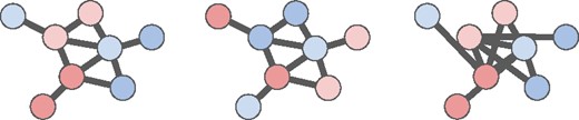
Left: Observed vertex-weighted graph $G=(V,E,w)$ with vertex colors indicating vertex weights. Center: A random vertex-weighted graph $G_w=(V,E,w\prime )$ with edges identical to G and permuted vertex weights. Right: A random vertex-weighted graph $G_d=(V,E\prime ,w)$ with vertex weights and degrees identical to G and permuted edges

2.3.2 Statistical test on dendrograms

We evaluate the statistical significance of our observed dendrogram T by comparing it to dendrograms from a null distribution $\mathcal{T}$ of dendrograms that we obtain by sampling from ${\mathcal{G}}_w,{\mathcal{G}}_w^{\ell }$ or ${\mathcal{G}}_d$⁠. Classic approaches to comparing dendrograms include the cophenetic distance (Sokal and Rohlf, 1962) and the Fowlkes-Mallows index (Fowlkes and Mallows, 1983). Both measures compare two clusterings by measuring how many objects are grouped together in both clusterings. However, in our application of altered subnetwork identification, we are typically interested in cuts of the dendrogram where most vertices are singletons, i.e. clusters of size 1. Neither of these two classic measures is appropriate in this case; therefore, we compare clusterings by comparing cluster sizes.

For a dendrogram T, we define

$$X_{\delta }=\underset{C\in C_{\delta }}{\max }\left|C\right|$$

(7)

as the size of the largest cluster $C\in C_{\delta }$ at a similarity threshold δ.

We quantify the deviation of the observed dendrogram T from a null distribution $\mathcal{T}$ of dendrograms at a similarity threshold δ as the ratio of the observed size of the largest cluster to the expected size of the largest cluster at δ. Let

$$Y_{\delta }=\frac{X_{\delta }}{\mathbb{E}[X_{\delta }]}$$

(8)

be a random variable for this ratio, where the expected value is computed over an appropriate null distribution $\mathcal{T}$ of dendrograms. Let $Y_{\text{max}}={\max }_{\delta }{Y}_{\delta }$ be the largest deviation, and let $y_{\text{max}}$ be the observed value of $Y_{\text{max}}$ on the observed dendrogram T. Note that while the maximum cluster size $X_{\delta }$ occurs at the root of the dendrogram, the maximum ratio $Y_{\text{max}}$ typically occurs at an intermediate value of δ between the root and the leaves.

We define

$$p=\text{Pr}(Y_{\text{max}}\ge y_{\text{max}}|\mathcal{T})$$

(9)

as the P-value for the largest ratio of the observed and expected cluster sizes across all similarity thresholds δ. Furthermore, we specify a representative clustering $C_{\text{max}}$ for the similarity threshold

$${\delta }_{\text{max}}=\underset{\delta }{\text{argmax}}{y}_{\delta }$$

(10)

that achieves the maximum observed ratio $y_{\text{max}}$⁠. Figure 4 illustrates this statistical test.

Fig. 4.

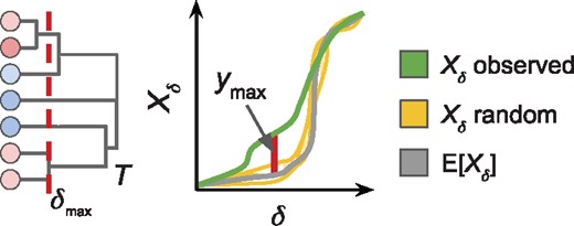
Left: Dendrogram T with similarity threshold δ of maximum deviation $y_{\text{max}}$⁠. Right: Maximum deviation $y_{\text{max}}$ between observed and expected largest cluster sizes

2.4 Consensus summarization for multiple datasets

In many biological applications, one may want to combine information from multiple vertex scores and multiple interaction networks. Vertices may be weighted with different statistical measures on individual genes, and interaction networks may be defined by different interactions (e.g. physical versus genetic) with the cancer sequencing application in Section 3 as one such example. Although one may build a single consensus network and consensus scores in advance, an alternative and useful approach (Leiserson et al., 2015) is to form a consensus of the resulting subnetworks, which can reduce network and score artifacts. We now define one such procedure.

Let $G_1,\dots ,G_t$ be a collection of vertex-weighted graphs corresponding to different combinations of interaction networks and vertex scores. For each such vertex-weighted graph $G=(V,E,w)$⁠, we find the clusters $C_{\delta }$ for a specific value of δ, e.g. $C_{\text{max}}$⁠, where δ may differ for each combination of network and scores. Let ${\lambda }_G(v)=1$ if v belongs to one of the non-singleton clusters of $C_{\delta }$ and ${\lambda }_G(v)=0$ otherwise. Let ${\mu }_G(u,v)=1$ if both u and v belong to the same non-singleton cluster of $C_{\delta }$ with $u,v\in E$ and ${\mu }_G(u,v)=0$ otherwise. Given a threshold $\ell$⁠, we define a consensus graph ${\overline{G}}_{\ell }=({\overline{V}}_{\ell },{\overline{E}}_{\ell })$⁠, where

$${\overline{V}}_{\ell }=\{v\in \widehat{V}:{\displaystyle \sum _{i=1}^t{\lambda }_{G_i}}(v)\ge \ell \},$$

(11)

$${\overline{E}}_{\ell }=\{(u,v)\in \widehat{V}\times \widehat{V}:{\displaystyle \sum _{i=1}^t{\mu }_{G_i}}(u,v)\ge \ell \}$$

(12)

with $\widehat{V}={\cup }_{i=1}^t{V}_i$⁠. This procedure extends to directed and weighted interactions with minor changes.

Many methods, including heinz, MUFFINN and NetSig, do not provide consensus procedures. HotNet2’s consensus procedure begins with ‘core’ sets of nodes found in the results for all networks and extends these sets iteratively with nodes found with fewer networks. In contrast, Hierarchical HotNet’s consensus procedure more simply considers the nodes and edges found in the results for multiple vertex-weighted graphs, further reducing artifacts by requiring more support for each prediction.

2.5 Implementation

We provide an implementation of Hierarchical HotNet in Python, where parts of Hierarchical HotNet are also implemented in Fortran to provide optional but significant performance improvements. Hierarchical HotNet is highly parallelizable and can be used with single-core machines, many-core machines and compute clusters. Our code, along with examples and experiments from this article, is available online at http://github.com/raphael-group/hierarchical-hotnet.

3 Results

We apply Hierarchical HotNet and other state-of-the-art methods to the problem of identifying significantly mutated subnetworks in cancer. In this application, each gene is assigned a score according to the frequency, or statistical significance, of the somatic mutations in the gene across a cohort of tumors. Methods for identifying altered subnetworks exploit the observation that driver mutations alter a limited number of biological functions and aim to identify significantly mutated subnetworks that might include both frequently and rarely mutated genes.

3.1 Data

We used two recent somatic mutation datasets and the most recent versions of several publicly available interaction networks.

3.1.1 Somatic mutation data

We used gene mutation scores derived from two sources: (i) frequencies of non-synonymous somatic mutations in genes across 10 206 tumors from 33 tumor types in the The Cancer Genome Atlas (TCGA) PanCanAtlas project (Ellrott et al., 2018; Weinstein et al., 2013); (ii) MutSig q-values (Lawrence et al., 2014) from 4 742 tumors across 21 tumor types. MutSig, like other statistical driver gene prediction methods, corrects for biases in somatic mutation frequencies due to gene length, regional variation in background mutation rate etc.

When computing mutation frequency scores, we removed hypermutated samples and genes such as TTN that are mutated in large numbers of samples but not identified as significantly mutated by MutSig. Table 2 summarizes the resulting datasets, and the supplement describes the complete sources and processing steps for each dataset.

Table 2.

Summary of the gene scores used in the analysis

Gene mutation scores	Number of scored genes	Number of samples	Number of tumor types
PanCanAtlas mutation frequency	19 057	9326	33
MutSig q-value	18 388	4742	21

3.1.2 Interaction network data

We created a HINT + HI interaction network by combining binary and co-complex interactions in HINT (Das and Yu, 2012) with high-throughput derived interactions from the HI network (Rolland et al., 2014). We also used the iRefIndex 15.0 (Razick et al., 2008) and ReactomeFI 2016 (Croft et al., 2014; Fabregat et al., 2016) interaction networks. We treated each network as undirected and unweighted (only Hierarchical HotNet is able to consider both directed and weighted interactions) and analyzed the largest connected subgraph in each network. Table 3 summarizes the resulting datasets, and the Supplementary Material describes the complete sources and processing steps for each dataset.

Table 3.

Summary of the interaction networks used in the analysis

Interaction network	Vertices	Edges	Density	M.D.	A.S.P.	Diameter
HINT + HI	15 074	182 088	0.00160	11	3.4	9
iRefIndex	17 136	408 688	0.00278	21	3.0	8
ReactomeFI	11 501	209 020	0.00316	13	3.4	13

M.D., median degree; A.S.P., average shortest path.

The high overlap of high-degree and high-scoring genes in each combination of gene scores and interaction network (see Table 4) reflects network ascertainment bias, where genes that are recurrently mutated in cancer are likely to have been studied more intensively, and thus have higher degree in interaction networks. This observation highlights the need to penalize or otherwise condition on degree for high-degree vertices.

Table 4.

Hypergeometric test P-values for overlap between the top 1% of genes ranked by indicated gene score and the top 1% of genes ranked by degree in each interaction network

	Mutation frequency	MutSig
HINT + HI	2.8 × 10–3	6.5 × 10–5
iRefIndex	4.1 × 10–6	2.3 × 10–12
ReactomeFI	1.1 × 10–5	9.1 × 10–14

3.2 Comparison of network methods on mutation data

We compared heinz, MUFFINN (DNmax and DNsum), NetSig, HotNet2 and Hierarchical HotNet using MutSig gene scores across three interaction networks: HINT+HI, iRefIndex and ReactomeFI interaction networks. When possible, we ran methods as prescribed in the published paper introducing the method; the Supplementary Material more fully describes these steps.

For such a comparison, one needs ground truth or a gold standard, but there is no gold standard list of cancer genes. There are various lists of known cancer genes, such as the COSMIC Cancer Gene Census (CGC) (Forbes et al., 2017; Futreal et al., 2004), but these lists are incomplete. Also, while a method’s ability to recover known cancer genes is suggestive of its ability to recover novel cancer genes, it is not a guarantee. In some cases, high recall of known cancer genes may reflect a method’s preference for well-studied (high-degree) genes and provide no assurance that the method’s novel discoveries are interesting. To address these issues in our comparison, we defined two complementary lists of cancer genes. First, we defined a list of known cancer genes using 676 genes from Tiers 1 and 2 of the COSMIC CGC. Second, we defined a list of candidate cancer genes as the set of non-CGC genes with below median degree in a network and MutSig gene scores q < 1. There are 519, 544 and 439 such candidate cancer genes in the HINT + HI, iRefIndex and ReactomeFI interaction networks, respectively. By definition, these candidate cancer genes are not known cancer genes, they are generally less studied because they have fewer known interactions, and they have some support as driver genes because they have MutSig gene scores q < 1.

We evaluated each method by computing its precision on the list of known cancer genes as well as its precision on the list of candidate cancer genes. Known and candidate cancer genes dominate the results of methods that score highly by both measures, and since these sets are necessarily disjoint, there is an inherent trade-off between them. Figure 5 shows the performance of each method according to these complementary measures. As an additional benchmark, we also computed the measures for genes with significant (q < 0.1) MutSig scores to show how network methods compare with gene scores alone.

Fig. 5.

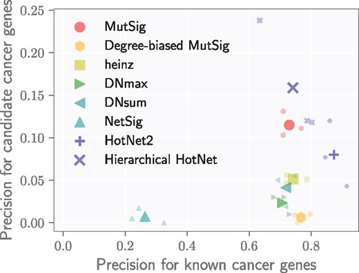
Precision on known cancer genes (x-axis) and on candidate cancer genes (defined in text; y-axis) for eight different methods using MutSig gene scores across three interaction networks. Smaller markers show the precision of a method on each network, and larger markers indicate the average precision of a method across networks

Hierarchical HotNet recovers larger proportions of both known and candidate cancer genes compared with other methods. All other network methods perform worse that the MutSig gene scores alone in identifying candidate cancer genes. HotNet2 identifies larger fractions of known cancer genes than MutSig but smaller fractions of candidate cancer genes. Like Hierarchical HotNet, HotNet2 also consider topology and scores jointly and penalizes high-degree genes. However, HotNet2 is less robust to complex network topology than Hierarchical HotNet and therefore less able to predict novel cancer genes, which we further describe in the following section.

heinz finds a slightly larger proportion of known cancer genes than MutSig but a much smaller fraction of candidate cancer genes. Its connectivity constraint provides modest improvements for known cancer genes by removing a few high-scoring genes that do not interact with other high-scoring genes, but this constraint introduces a bias toward high-degree nodes (see Table 5) that reduces its ability to identify less studied genes.

Table 5

Median degrees of vertices identified by each method on different interaction networks, with methods sorted from smallest to largest degree

Methods	HINT +  HI degree	iRefIndex degree	ReactomeFI degree
NetSig	27	54	46
Hierarchical HotNet	33.5	106	48
MutSig	29	95	90
HotNet2	32	92	95.5
heinz	40.5	118	104.5
DNmax	56	154	121
DNsum	53	170	124
Degree-biased MutSig	54	175	128

MUFFINN identifies similar fractions of known cancer genes as MutSig but smaller numbers of candidate cancer genes, demonstrating an even stronger preference for high-degree nodes. MUFFINN’s DNmax and DNsum scores take the maximum and sum, respectively, of the scores of their neighbors, favoring genes with large network neighborhoods.

We created a degree-biased version of MutSig (see the Supplementary Material for details) that reprioritizes genes using a weighted combination of MutSig score and degree, which modeled network ascertainment bias to recover more known cancer genes at the expense of candidate cancer genes. As a result, it has similar performance to both heinz and MUFFINN.

NetSig finds smaller proportions of known and candidate cancer genes than MutSig. The NetSig statistic intentionally omits a gene’s score when evaluating its network neighborhood, thus reducing NetSig’s recovery of known cancer genes with high MutSig scores. However, we found that most NetSig genes (380/463 distinct genes) have MutSig scores of q = 1, thus having little support for their recurrent mutation across the cohort as candidate cancer genes. Also, while NetSig’s statistical test attempts to condition on vertex degree, we find that NetSig reports several high-degree nodes, such as UBC, that are less likely to be cancer genes.

3.3 Hierarchical HotNet hierarchies and consensus results

Beyond predicting known and candidate cancer genes, Hierarchical HotNet also builds hierarchies of significantly mutated subnetworks and constructs consensus subnetworks across multiple network topologies and gene scores. This section describes its results on three distinct interaction networks (HINT + HI, iRefIndex and ReactomeFI) and two distinct sets of genes scores (PanCanAtlas mutation frequency scores and MutSig q-value scores). Hierarchical HotNet’s results were statistically significant (P < 0.01) on each of the six resulting vertex-weighted graphs.

Hierarchical HotNet identified gene sets that had strong overlap with biological pathways that are implicated in cancer. For example, Figure 6 shows part of the Hierarchical HotNet hierarchy for the ReactomeFI interaction network and TCGA PanCanAtlas mutation frequency scores. This part of the Hierarchical HotNet hierarchy overlaps well with the Notch signaling pathway, containing the Notch genes NOTCH1, NOTCH2, NOTCH3, NOTCH4, JAG1, JAG2 and DLL3 as well as the COSMIC CGC genes CPEB3 and RB1 that interact with Notch pathway mutations.

Fig. 6.

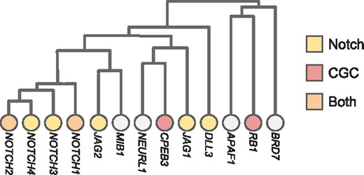
Branches of the Hierarchical HotNet hierarchy for the ReactomeFI interaction network and TCGA PanCanAtlas mutation frequency gene scores, where Notch signaling pathway and COSMIC CGC genes are indicated (branch heights roughly to scale)

Across these interaction networks and gene scores, Hierarchical HotNet identified the consensus subnetworks ${\overline{G}}_2$ (see Section 2.4) with 128 genes and 223 interactions supported by multiple significantly mutated subnetworks within their respective hierarchies. See the Supplementary Material for a full list of Hierarchical HotNet consensus genes, biological process and pathway annotations of the Hierarchical HotNet genes and a network view of the Hierarchical HotNet consensus subnetworks.

Many of the Hierarchical HotNet consensus results are known cancer genes, and the Hierarchical HotNet consensus subnetworks contain parts of many canonical cancer pathways, including the Notch (Rizzo et al., 2008), p53 (Vazquez et al., 2008), PI(3)K (Liu et al., 2009; Yuan and Cantley, 2008), Ras/Raf (Roberts and Der, 2007) and Rb (Nevins, 2001) signaling pathways. They also contains gene sets with more recent implications in cancer, including parts of the BAP1 (Carbone et al., 2013), CBFB (Banerji et al., 2012) and SWI/SNF (Wiegand et al., 2010) complexes. Moreover, the Hierarchical HotNet consensus results contain novel predictions that may be of interest for further study, including the possible tumor suppressors RASA1 and SERPINB5. Hierarchical HotNet also identifies a subnetwork of protein kinase D1 genes (PKD1 and PKD2) with known roles in cell proliferation and other cancer hallmarks (Sundram et al., 2011). An additional subnetwork includes several putative cancer genes that interact but do not otherwise have a clear relationship to one another: MERTK is a receptor tyrosine kinase that may activate several downstream oncogenic pathways (Cummings et al., 2013), VWF has recently been implicated in angiogenesis and apoptosis (Franchini et al., 2013) and PROS1 may be a marker for aggressive prostate cancer (Saraon et al., 2012).

Since HotNet2 also provides consensus results, we compared Hierarchical HotNet’s consensus subnetworks with HotNet2’s consensus subnetworks on the same data. Although Hierarchical HotNet results were statistically significant (P < 0.01) on each dataset, HotNet2 had statistically insignificant (P ≥ 0.05) results for mutation frequency scores on the iRefIndex or ReactomeFI networks. For the rest of the section, we compare the recall and precision of these methods for known cancer genes because a consensus comparison of candidate cancer genes is more complicated as these sets differ across networks and gene scores.

Figure 7 summarizes the overlap of the Hierarchical HotNet and HotNet2 consensus results with COSMIC CGC gene list. Hierarchical HotNet and HotNet2 recover 37 of the same genes, including 30 COSMIC CGC genes. However, Hierarchical HotNet identifies 91 genes that HotNet2 does not, including 27 CGC genes. These 27 genes include the well known cancer genes APC, CTNBB1, PTEN, TP53 and VHL. Each of these genes is significantly and recurrently mutated, but these well studied genes tend to have more reported interactions in more recent interaction networks, and the larger and denser networks in this analysis frustrates HotNet2’s less robust subnetwork selection procedure. Conversely, HotNet2 predicts 52 genes that Hierarchical HotNet does not, including three CGC genes: KEAP1, NFE2L2 and RSPO3. Hierarchical HotNet’s more aggressive consensus procedure eliminates the interacting partners KEAP1 and NFE2L2, but RSPO3 is absent from both the HINT + HI and ReactomeFI networks, so its loss in Hierarchical HotNet is more predictable.

Fig. 7.

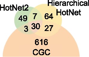
Venn diagram summarizing the overlap of HotNet2 and Hierarchical HotNet consensus results with the COSMIC CGC genes

Overall, Hierarchical HotNet identifies more COSMIC CGC genes than HotNet2 (57 versus 33, respectively), giving it nearly twice the recall (0.087 versus 0.051) with higher precision (0.445 versus 0.371, respectively) than HotNet2 (see Fig. 7 and Table 6). Hierarchical HotNet’s higher recall and precision are primarily attributable to Hierarchical HotNet’s ability to identify significantly mutated subnetworks across biological scales in its hierarchy of subnetworks and more aggressive consensus procedure.

Table 6.

Overlap of HotNet2 and Hierarchical HotNet consensus results with the COSMIC CGC genes

Consensus results	Total genes	CGC genes	CGC recall	CGC precision
HotNet2	89	33	0.051	0.371
Hierarchical HotNet	128	57	0.087	0.445

In practice, Hierarchical HotNet is more flexible, more robust and less computationally intensive (CPU time, memory usage and storage space) than HotNet2. For these results, the entire HotNet2 pipeline required a few days of compute time on a modern, many-core machine while the entire Hierarchical HotNet pipeline required a few hours.

4 Discussion

In this article, we introduce a novel computational method, Hierarchical HotNet that simultaneously combines network interactions and vertex scores to construct a hierarchy of high-weight, topologically close subnetworks.

Applied to cancer genomics data, Hierarchical HotNet builds a hierarchy of highly mutated subnetworks in a PPI network. Hierarchical HotNet outperforms several state-of-the-art computational methods on recent datasets in terms of recovering known and candidate cancer genes, addressing several important issues in current network-based methods for identifying altered subnetworks, including ascertainment bias (i.e. bias toward high-degree nodes) and statistical significance testing. In particular, Hierarchical HotNet is a simpler but more robust method than our earlier HotNet2 algorithm (see Supplementary Material for a more detailed comparison), removing parameters, reducing computational costs and improving predictions. Applied to multiple interaction networks and cancer mutation datasets, Hierarchical HotNet identifies many known and putative cancer genes. Further testing of these novel predictions may provide additional insight into cancer biology.

There are multiple avenues for extending Hierarchical HotNet. Hierarchical HotNet can be understood as part of general framework for identifying clusters of high-weight, topologically close vertices. As such, Hierarchical HotNet is a modular method; different similarity measures, clustering algorithms or test statistics may be more appropriate for different datasets, and each of these parts can be changed as the application demands or curiosity dictates. This modularity is strength of Hierarchical HotNet that should allow it to be applied broadly.

It is also possible to adapt Hierarchical HotNet to use categorical or vector-valued attributes instead of scalar-valued weights. For example, one could define a new mutation similarity matrix using the statistical significance of mutually exclusive or co-occurring mutations between pairs of genes. Leiserson et al., (2016) use this similarity matrix either directly with Hierarchical HotNet or after combining it with the topological similarity matrix (1) to create a new joint similarity matrix.

There is also a larger question about similarity measures on vertex-weighted graphs and what properties such measures should have. For the example, there is an interplay between the contributions from network topology and vertex weights, and an ideal method would attempt to quantify or balance these contributions to the discovery of a method’s results. Hierarchical HotNet acknowledges this interplay, and its framework provides opportunities to ascertain, e.g. if either network topology or vertex weights dominate the Hierarchical HotNet results. Additional study of similarity measures on vertex-weighted graphs would be useful in the design of new methods for altered subnetwork discovery.

Funding

This work is supported by a US National Science Foundation (NSF) CAREER Award [CCF-1053753] and US National Institutes of Health (NIH) grants [R01HG007069 and U24CA211000 to B.J.R.]. The results shown here are in part based upon data generated by the TCGA Research Network http://cancergenome.nih.gov/ as outlined in the TCGA publications guidelines.

Conflict of Interest: B.J.R. is a co-founder and board member of Medley Genomics and M.R. is a contractor for Medley Genomics.