TiSAn: estimating tissue-specific effects of coding and non-coding variants

Abstract

Motivation

Model-based estimates of general deleteriousness, like CADD, DANN or PolyPhen, have become indispensable tools in the interpretation of genetic variants. However, these approaches say little about the tissues in which the effects of deleterious variants will be most meaningful. Tissue-specific annotations have been recently inferred for dozens of tissues/cell types from large collections of cross-tissue epigenomic data, and have demonstrated sensitivity in predicting affected tissues in complex traits. It remains unclear, however, whether including additional genome-scale data specific to the tissue of interest would appreciably improve functional annotations.

Results

Herein, we introduce TiSAn, a tool that integrates multiple genome-scale data sources, defined by expert knowledge. TiSAn uses machine learning to discriminate variants relevant to a tissue from those with no bearing on the function of that tissue. Predictions are made genome-wide, and can be used to contextualize and filter variants of interest in whole genome sequencing or genome-wide association studies. We demonstrate the accuracy and flexibility of TiSAn by producing predictive models for human heart and brain, and detecting tissue-relevant variations in large cohorts for autism spectrum disorder (TiSAn-brain) and coronary artery disease (TiSAn-heart). We find the multiomics TiSAn model is better able to prioritize genetic variants according to their tissue-specific action than the current state-of-the-art method, GenoSkyLine.

Availability and implementation

Software and vignettes are available at http://github.com/kevinVervier/TiSAn.

Supplementary information

Supplementary data are available at Bioinformatics online.

1 Introduction

Whole genome sequencing (WGS) is assuming a role as the technology of choice for an increasing number of genetic studies. The vast majority of the information yielded by WGS resides in non-coding and poorly-characterized regions of the genome. Recent work in annotating non-coding variation has shown that multiple levels of information—integrated using machine learning algorithms—are required to capture the diverse regulatory potentials in these regions (Ionita-Laza et al., 2016; Kellis et al., 2014; Kircher et al., 2014; Quang et al., 2015). However, current state-of-the-art variant annotation methods predict generic pathogenicity, largely avoiding the question of which tissues, organs and systems are most likely susceptible to a particular genetic variation. Projects such as the Genotype-Tissue Expression (GTEx) repository (GTEx Consortium, 2015) and the NIH Roadmap Epigenomics (RME) Mapping Consortium (Bernstein et al., 2010), provide clear evidence that a given variant will not necessarily have the same impact on gene expression in different tissues or cell types. Recently proposed approaches, such as GenoSkyline (Lu et al., 2016), have employed cross-tissue methylation levels to annotate genetic variations. However, such methods are limited because they were trained using only data uniformly collected across a wide variety of tissues, omitting potentially informative features derived from databases providing unique, tissue-specific information. Such approaches emphasize performance over many tissues, rather than a specific tissue.

In this work, we introduce Tissue-Specific Annotation (TiSAn), which combines the power of supervised machine learning with tissue-specific annotations, including genomics, transcriptomics and epigenomics (http://github.com/kevinVervier/TiSAn for the latest version). We describe a general statistical learning framework in which researchers can derive a nucleotide-resolution score for the tissues they focus on. We foresee TiSAn’s application as a complement for existing scores that measure generic variant deleteriousness, like CADD or DANN. This combination makes it possible to infer which variants may be most damaging in the context of the tissue of interest. As a proof of principle, we apply our methodology to two human tissues—brain and heart—and we have made available pre-computed genome-wide scores for these tissues.

2 Materials and methods

2.1 Training set definition

We identified multiple sources of training examples with respect to a given tissue T. For deriving a genome-wide predictor, the training set needed to cover both coding and non-coding loci, but also loci related (positive examples) and unrelated to T (negative examples).

Two types of public databases were used to derive training sets:

• Genotype array loci: Disease-related loci were identified in consortium-developed arrays, designed for targeting specific disorders, such as MetaboChip (Voight et al., 2012) for cardiovascular diseases or Illumina Infinium PsychArray Beadchip for psychiatric disorders. Genotyped single nucleotide polymorphisms (SNP) were sorted by confidence level into three classes. First, replication SNPs were selected as follow-up for top association signals from the largest available genome-wide association studies (GWAS) meta-analysis, and contain tissue-related variants (positive examples). Then, fine-mapping SNPs represent associated haplotypes identified in preliminary studies. Finally, backbone SNPs include sex-specific markers, Major histocompatibility complex region and other population variation, which we consider as negative examples if they meet a minimal CADD threshold described in Section 2.9. To ensure the highest quality of positive labels, we only considered the first category in our analysis, as positive examples.

• Large intergenic non-coding RNAs: Large intergenic non-coding RNAs (lincRNAs) represent a well-studied group of non-coding elements known to regulate gene transcription in a tissue-specific manner (Popadin et al., 2013). Databases such as LincSNP (Ning et al., 2014), contain disease-related variants that occur in lincRNA loci. This is an important source of non-coding training examples, since non-coding variants are generally less functionally characterized than coding variants. After defining a list of tissue-related disorders, we divided this database into two subsets: one related to tissue T (positive examples) and one containing background variants (negative examples), i.e. randomly sampled deleterious variants not related to the tissue at hand. This way, we enriched the training set with putatively functional non-coding positions.

We endeavored to ease the training set selection process for users interested in training their own models, by developing a companion tool called TiSAn-build (http://github.com/kevinVervier/TiSAn/tree/master/TiSAn-build). Using this Shiny (Chang et al., 2017) graphical user interface (GUI), the user can select training positions based on a list of keywords and disease names (Supplementary Fig. S22). The number and breakdown of training examples used for TiSAn brain and heart models can be found in Supplementary Table S1. After selection of positive and negative examples, we ensured there was no selection bias between the two groups that would lead to poor generalizability of the classifier. For both brain and heart models, half of the training examples were found within the proximity of a gene (±10 kb) and the remaining 50% were in intergenic regions, with no detectable difference in the spatial distribution between positive and negative examples. The variants found in genic regions covered 7219 and 7625 different genes in the brain and heart training sets, respectively. No significant difference in terms of minor allele frequency (MAF) distribution between positive and negative examples was observed (brain: Wilcoxon test P = 1, average MAF = 0.14, heart: Wilcoxon test P = 0.8, average MAF = 0.4). No significant difference was observed in terms of variant pathogenicity (CADD Phred score) distribution between positive and negative examples (brain: Student’s test P = 1, average CADD = 3.5, heart: Student’s test P = 0.66, average CADD = 4.1).

2.2 Feature extraction

We represent each genomic position in a functional space defined by hundreds of different annotations. In the following, we describe how such signal can be extracted using publicly available datasets, and provide a comprehensive list of variables used in this study in Supplementary Table S2. Most of the feature extraction process can be extended to a wide variety of tissues (Supplementary Table S3), and we have developed a companion tool, called TiSAn-build, aiding users in extracting features for their own models. Users can assemble tissue-specific signal from eQTL (Supplementary Fig. S19), DNA methylation (Supplementary Fig. S20) or literature databases (Supplementary Fig. S21) which the machine learning algorithm uses as reference annotations to extract features on training examples.

2.2.1 Motifs in short nucleotide sequences

Nucleotide frequencies are linked to overall regulatory activity (G/C content), and patterns in nucleotide k-mers are the basis of transcription factor binding site detection (Zhou and Troyanskaya, 2015). Specific patterns have been recently identified to be tissue-specific (Zhong et al., 2013), and we incorporate this information by computing frequencies for all n-nucleotides [$n\in (1,2,3,4)$], found within a ±500 base pair neighborhood around a given genomic position x.

2.2.2 Distance to annotations

We model the impact of a known annotation on a given position x, as a decreasing function of their distance. The comparison between four different distributions found that the Weibull distribution was the most stable across the considered features (Supplementary Table S4). Therefore, in the following paragraphs, the distance is measured as:

$$d(x,anno)=\left(\frac{\beta }{\alpha }\right){\left(\frac{|x-anno|}{\alpha }\right)}^{\beta -1}\hspace{0.17em}\text{exp}\left(-{\left(\frac{|x-anno|}{\alpha }\right)}^{\beta }\right),$$

where anno refers to a known annotation position, α is a scale factor and β is a shape parameter. Parameter fitting was performed separately for each annotation, using the MASS R package (Venables and Ripley, 2002).

2.2.3 Expression quantitative trait loci

Links between disease traits and tissue-specific gene expression have been reported in studies using the GTEx dataset (GTEx Consortium, 2015). For each genomic location, we extract features based on a position’s distance to known eQTL for tissue T, as well as for other tissues. The Weibull distribution was used for modeling the minimal distance to a GTEx eQTL (Supplementary Fig. S1). We also derive Boolean features for whether the genomic position is at the exact location of a GTEx eQTL, which puts more weight on known eQTL.

2.2.4 Literature mining for tissue-related genes

Although gene expression shows variation across tissues, definitive lists of tissue-specific genes are limited. It has already been shown that text mining techniques may help to extract relationships between genes and disease traits (Liu et al., 2015). Therefore, we adapt such methods to identify genes reported to be associated with tissue T, in the PubMed database (May 2016 gene2ID database). Genes co-cited at least 3 times in publication’s title/abstract with the tissue name (e.g. ‘brain’ or ‘heart’) are kept as tissue-related genes (Collier et al., 2015). For each genomic location, we extract features based on how close the position is to tissue-related genes. The Weibull distribution is used for modeling the minimal distance to a gene (Supplementary Fig. S2). We also derive a Boolean feature for whether or not the genomic position x is within the range of a tissue-related gene, which puts more weight on positions in regions well-supported by literature for its association with the tissue of interest. When training the brain model under the Weibull distribution assumption, we observed that around 1000 tissue-related genes represented enough genome coverage to derive a feature based on the proximity between a locus x and a gene. Lists of genes identified as tissue-related are provided in Supplementary Data S1 (1185 brain genes) and Supplementary Data S2 (1721 heart genes).

2.2.5 Differentially methylated regions

Epigenomics, and, in particular, methylation profiles, have been integrated to explain tissue-specific regulatory mechanisms (Miller et al., 2016). We use the Weibull distribution approach for modeling the minimal distance to a methylated region found in the RME database (Supplementary Fig. S3). If the considered position x belongs to a methylated region characterized in the RME project, we also note the average methylation level for samples from the tissue of interest T, and other samples.

2.2.6 Additional tissue-specific resources

In contrast to approaches that rely mostly on RME and/or GTEx, we also consider tissue-specific datasets made available by research projects focusing on a single tissue. For the brain model, we integrate developmentally differentially methylated positions (dDMPs) (Spiers et al., 2015) found in the fetal brain, and derive features based on the distance between and the closest dDMP. For the heart model, we use the Heart Enhancer Compendium database (Dickel et al., 2016) to identify heart development candidates, and we use the distance to the closest fetal development enhancer as a training feature for TiSAn heart model.

2.3 Supervised machine learning model training

Considering the aforementioned training sets, we utilized machine learning approaches, such as logistic regression (glm R package), linear support vector machine (libLineaR R package) and random forest (randomForest R package) (Lischke et al., 1998), and compared them based on their 10-fold cross-validated performance (herein, area under the receiver operating characteristic curve, AUC), and selected the random forest algorithm to train the final model (Supplementary Table S5). Using cross-validation, we optimize random forest hyper-parameters and build a model with 1000 trees, where each tree is trained on a bootstrapped sample of the training set, and all the 360 variables are considered (instead of the default value $\sqrt{360}\sim 19$⁠). The leaf node size is set, by default, as equal to one, meaning that each root-leaf path is predicting a single example.

2.4 From class probability to rescaled odds ratio

Current variant annotation approaches often consider the raw class probability as their functional score, requiring an additional tuning/thresholding step from the user. Herein, we propose to rescale the classifier output into a ready-to-use score. First, we define an optimal cutoff value on the class probability (Supplementary Figs S4A and S5A), as the smallest value which reaches a false discovery rate (FDR) of 10%. For instance, this threshold is equal to 0.48 for the brain model and to 0.67 for the heart model. Using FDR as a threshold also accounts for potential mislabeling in the training data, especially in the background/negative examples set. We then rescale the filtered probability to a score between 0 and 1, using the formula:

$$\text{max}\left(0,1-thresh-\frac{\mathbb{P}\left(x\cancel{\notin }tissue\right)}{\mathbb{P}\left(x\in tissue\right)}\right).$$

The main advantage here is to standardize predictive models, and push non-tissue-related loci to a score strictly equal to 0 (Supplementary Figs S4B and S5B and S18).

2.5 Reference genome

Analyses performed in this study used the hg19 reference genome.

2.6 GTEx transcriptome data for 44 tissues

Median gene expression data were downloaded from the GTEx portal (version 6), and are measured using Reads Per Kilobase, per Million mapped reads (RPKM). We used the median RPKM, as it measures expression at the entire gene scale, and allowed us to correlate expression with a gene-level median TiSAn score. We acknowledge that the use of raw expression data may contain biological and technical confounders. We therefore limited the analysis to the 17 803 genes that were used in the original GTEx eQTL study, after being fully processed, normalized and filtered.

2.7 ENIGMA genome-wide association for brain regions volume

Genome-wide association summary statistics from the ENIGMA2 study (Hibar et al., 2015) were downloaded from www.enigma.ini.usc.edu. For the four considered brain regions (accumbens, amygdala, caudate and hippocampus), we annotated each of the 974 045 intergenic loci with a distance to the closest gene of at least 10 000 bp with Tisan-brain.

2.8 GWAS prioritization in coronary artery disease (CAD-GWAS) cohort

CARDIoGRAM consortium GWAS meta-analysis summary statistics for 8 443 810 SNPs were downloaded from http://www.cardiogramplusc4d.org. We carefully removed positions that were found both in the TiSAn training and the GWAS, to avoid an overly-optimistic estimation of performance. A comparison between the TiSAn score and association strength (Fig. 4) was obtained by binning coronary artery disease (CAD)-GWAS SNPs in 100 percentile bins on reported GWAS P-value. Average score gain is measured for top 1% variants (Bin 1) by comparing their scores against the remaining 99% of the SNPs. Then the top 2% variants (Bins 1 and 2) are compared against the remaining 98%, and so on, until merging all the data, which corresponds to the comparison between 99% of the data against the 1% variants with the highest P-value. We derived confidence intervals for both TiSAn and GenoSkyline by random permutations on the GWAS P-values. When ranking variants that might have an impact on the trait, we filtered variants not predicted as tissue-related by either TiSAn (zero score), or by GenoSkyline (score <0.15).

2.9 Variant enrichment in the vicinity of ASD genes

Variants found in 960 Simons Simplex Collection (SSC) individuals—including probands and parents—were filtered based on their pathogenicity using CADD score. We estimated different threshold values for coding (>15) and non-coding (>10.7) variants to account for systematic bias in CADD predictions. Those values correspond to the top 10 percentile found in the 1000 Genomes data. We also focused the analysis on variants found in ±50 000 bp windows around well-supported autism spectrum disorder (ASD) genes with more than 20 citations in the June 2016 SFARI gene list at http://gene.sfari.org/autdb/HG_Home.do (Supplementary Table S6). The same filters were applied to variants found in 1000 Genomes (1KG) European ancestry population (Phase 3). We carefully removed positions that were found in both the TiSAn training and the sequencing variant call sets (SSC and 1KG), to avoid an overly optimistic estimation of performance. We also controlled for potential linkage disequilibrium (LD) between training data and validation variants. LD correlation (R-squared) was estimated from 1000 Genomes European population (CEU) allele frequencies using SNAP proxy search (www.archive.broadinstitute.org/mpg/snap/ldsearch.php). For each validation locus (positive or negative), we considered the maximal correlation value with the training set loci. The distributions obtained for positive and negative examples were compared, and correlation for positive examples was not found to be significantly higher (Wilcoxon rank test: P = 0.9971, average LD positive = 0.92, average LD negative = 0.93). Coding and non-coding variants were separated based on their RefSeq (O’Leary et al., 2016) function annotation. The relative gain in average score (Fig. 3A and B) was calculated by computing the difference between average functional score in SSC and in 1KG for coding and non-coding variants. Cumulative score enrichment for SSC over 1KG variants (Fig. 3C) was obtained by binning both SSC and 1KG variants based on their functional score, in 5 percentile groups. Then, the proportion of SSC SNPs and 1KG variants present in each bin was computed, and summed in a cumulative way, from the top 5% bin to all the data (from left to right on the figure).

2.10 Transcription factor binding site enrichment in tissue and cell type

The ENCODE project provides a large repository for Transcription factor binding site (TFBS) locations in various cell type contexts. Here, we assembled two databases, both available as UCSC Genome Browser tracks, factorbookMotifPos (from factorbookMotif track), which contains the location of more than 2 million TFBS across the genome, and EncodeRegTfbsClustered (ENCODE Regulation ‘Txn Factor’ track), which provides information regarding the cell types where TFBS were observed. Overlapping the two databases resulted in 1 514 086 unique TFBS found binding 53 different TF structural families. For each of those TFBS, we expanded their location using a ±500 base pair window centered on the site, and TiSAn heart and brain score profiles were extracted from these windows. Scores were centered and scaled around the center value and show the actual score enrichment along the window. An average profile was computed for all TF structural families and cell types.

2.11 TiSAn use case

The main application for TiSAn involves the annotation of large sets of variants, and we recommend the use of scalable tools, such as vcfanno (www.github.com/brentp/vcfanno) to accomplish this annotation. On the other hand, examination of one or a handful of loci can also be helpful in gaining insights about what features are driving a prediction. Therefore, we developed a GUI tool called TiSAn-view, where features extracted for a single locus are displayed (Supplementary Fig. S6). Users simply need to upload a list of genetic loci (e.g. in bed format), and choose the TiSAn to use. Tutorial and vignettes are available on http://github.com/kevinVervier/TiSAn.

2.12 Software availability

• Genome-wide TiSAn score databases (brain and heart) are available in bed format at http://www.flamingo.psychiatry.uiowa.edu/TiSAn. We have also made publicly available the two companion tools (TiSAn-build and TiSAn-view) at http://github.com/kevinVervier/TiSAn.

• GenoSkyline approach: we downloaded brain and heart models from (www.genocanyon.med.yale.edu), in November 2016.

• CADD: Deleteriousness annotations were performed using CADD v1.3 (current version) at http://cadd.gs.washington.edu

• DANN annotations were downloaded in April 2015 (original version) at http://cbcl.ics.uci.edu/public_data/DANN

3 Results

3.1 Machine learning for predicting tissue-specific functional annotation

The design of TiSAn models is outlined in Figure 1 (details in Section 2). Taking advantage of publicly available datasets (GTEx Consortium, 2015; Bernstein et al., 2010), we extracted more than 350 different genome-wide variables that were used to describe two large sets of disease-related loci. Training a supervised machine learning model requires positive and negative examples: herein, positive examples were nucleotide positions that had been previously linked to a tissue-specific disease, and negative examples were variants that had no established link to the tissue-specific disease in question. Predictive models were trained on the labeled datasets and optimized to achieve high discrimination of tissue-specific loci (Supplementary Figs S4 and S5). Herein, a score equal to 1 indicates a position strongly associated with the tissue, whereas a score of 0 means no association at all; such a position is usually discarded in subsequent analysis.

Fig. 1.

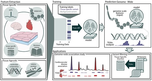
TiSAn framework overview. Each nucleotide position in the genome is annotated with multiple types of genome-scale information, such as sequence content, methylation level, proximity to genes, etc. (see Section 2). This information is extracted for training sets, comprised of deleterious variants with or without an association with the tissue of interest. Using supervised machine learning, specifically a Random Forest (RF), a predictive model combines each feature based on its ability to predict whether a position will be functionally associated with the tissue of interest. Model output consists in a tissue-specific functional score ranging from no functional relevance to the tissue (0) and strong functional relevance to the tissue (1). This score can then be used, for instance, to filter down large lists of candidate variants for further investigation, or to isolate the contribution of different tissues to a complex trait

3.1.1 Impact of algorithm hyper-parameters

Feature group importance. The cross-validation procedure indicated a random forest as the most accurate approach for the tissue-specificity task. Interestingly, this analysis suggested that using all the features when considering potential splits leads to superior performance, with the optimal mtry parameter being equal to the total number of features. In order to identify the most informative features, we compared the contribution of each feature group to the model’s accuracy, by training suboptimal models with features restricted to a single group. Notably, we found that eQTL are the most informative features for both brain and heart models, whereas DNA methylation shows limited performance (Supplementary Fig. S7). Additional tissue-specific epigenome data (e.g. H3k4me1) were found to have a negligible impact on performance (Supplementary Fig. S8), suggesting that the signal in RME consolidated epigenomes present in TiSAn models is sufficient.

Feature interactions. We identified combinations of features that were likely to increase model accuracy using an iterative Random Forest scheme (Basu et al., 2018). For the brain model, we observed a strong interaction between GC content and proximity with brain genes. In the heart model, interactions between heart eQTL and heart enhancers were the main contributors. A complete list of stable interactions is given in Supplementary Table S7.

Training set and learning curve. The number of training examples also has an impact on model performance (Supplementary Fig. S9). We found that the current training set size for both brain and heart models achieves the optimal trade-off between required labeled examples and model predictive power.

3.1.2 Region-based analysis

In addition to cross-validation performance, we assessed our models’ generalization by holding out two genome regions from the training sets, and confirmed there was no LD correlation between the training set and the tested regions. The 16p11 region (from position 28M to 31M) has been extensively studied in neurodevelopmental disorders, such as ASD (Weiss et al., 2008). The 9p21 region (from position 19.9M to 25.4M) has been associated with cardiovascular disease (Gong et al., 2014). We extracted the TiSan brain and heart scores within the two regions at a 1 kb resolution, and reported tissue-specific enrichment in Supplementary Figure S10. As expected, the brain score is significantly higher than the heart score in the 16p11 region (paired Student’s $P=1.38\times {10}^{-12}$⁠), whereas the heart score is significantly higher in the 9p21 region (paired Student’s $P=1.21\times {10}^{-127}$⁠). Finally, we also used the held-out labeled loci in those regions to estimate the TiSAn models’ sensitivity. Predictions with the brain model showed an AUC of 0.99 for the 16p11 region, and predictions with the heart model showed an AUC of 0.86 for the 9p21 region. These values were comparable to the observed cross-validated AUC for the corresponding models, supporting TiSAn’s generalizability.

3.2 Tissue signal detection in non-disease traits

Here we demonstrate that the TiSAn score can identify functional, tissue-specific variants that are not necessarily disease-related. First, we considered 44 tissues characterized by RNA-seq, from the GTEx project, including 2 heart tissues (atrial appendage and left ventricle), and 10 brain tissues. We observed correlation between the measured gene expression and the average corresponding TiSAn score both for gene and flanking regions (Supplementary Fig. S11). We found that TiSAn-brain is strongly associated with 9 out of 10 brain tissues, and TiSAn-heart shows enrichment for not only heart tissues, but also in liver and pancreas, which is reasonable given their known roles in diseases that are risk factors for cardiovascular disorders, such as hypercholesterolemia and diabetes. We also evaluated TiSAn’s capability to properly annotate intergenic loci associated with brain volume. While not a disease trait, brain volume has been associated with various neurodevelopmental and psychiatric disorders (van Erp et al., 2016). ENIGMA GWAS found statistical association between a large set of genetic variations and brain volume (Hibar et al., 2015). Figure 2 shows the correlation between the TiSAn brain score obtained for a locus and its association with brain volume. In the four considered brain regions, we observe the strongest signal for the loci within the top 5% GWAS associations, confirming a role for non-coding variation in a non-disease trait. The lack of a similar signal from the TiSAn heart model suggests good specificity (Supplementary Fig. S12). Interestingly, none of the generic pathogenicity scores [CADD (Kircher et al., 2014) and DANN (Quang et al., 2015)] detected a comparable enrichment around the stronger GWAS hits for any brain region (Supplementary Figs S13–S16). This suggests that TiSAn is uniquely able to capture functional, tissue-specific variation that is not necessarily pathogenic.

Fig. 2.

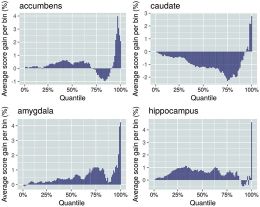
TiSAn-brain annotation of intergenic loci associated with brain volume. Each of 974 045 ENIGMA loci was binned into 100 percentile groups, based on the statistical association strength with brain volume. For each bin, the average TiSAn-brain score enrichment was computed with respect to the average score across the entire set of loci. The right part of each panel corresponds to loci with stronger associations with brain region volume

In the following, we demonstrate TiSAn performance in three different settings: (i) evaluating tissue-specific enrichment in case-control cohort, (ii) enhancing discovery in a genome-wide association study (GWAS) and (iii) identifying tissue-specific transcription factors. We also make practical comparisons to a recently proposed tool, GenoSkyline (Lu et al., 2016) that provides a genome partition in terms of functional segments using only methylation data. Our approach aims to provide functional prediction at the single nucleotide resolution, because variants found in large predicted functional blocks (as is the case in GenoSkyline) may in fact have different functional effects.

3.3 Brain-specific variant prioritization in a sample with familial risk for autism

3.3.1 Genome-wide enrichment for brain-related variations in affected individuals

The SSC (http://base.sfari.org) provides WGS for one of the largest ASD cohorts currently available. We hypothesized that deleterious genetic variation (see definition in Section 2) found in the vicinity of ASD-related genes would show higher enrichment in terms of brain-related functional consequences (as measured by the TiSAn-brain and GenoSkyline-brain scores) in the SSC compared to the 1000 Genomes (1KG) (1000 Genomes Project Consortium, 2012). We further assessed enrichment using the respective heart-specific scores as a form of negative control, since the cardiovascular system has not been found to be a major etiological contributor to ASD. In this analysis, the TiSAn-brain score showed the only positive tissue-specific enrichment, over 50% for coding variants (Fig. 3A) and around 10% for non-coding variants (Fig. 3B). Notably, there was a significant difference between TiSAn brain and heart scores (Wilcoxon signed-rank test, $P<2\times {10}^{-16}$⁠), suggesting effective tissue specificity, which was not observed for GenoSkyline models (Wilcoxon signed-rank test, P = 0.351). Interestingly, we did not observe a differential enrichment between SSC family members (proband, father, mother and sibling), suggesting a familial genetic burden for autism (F-test, P = 0.28).

Fig. 3.

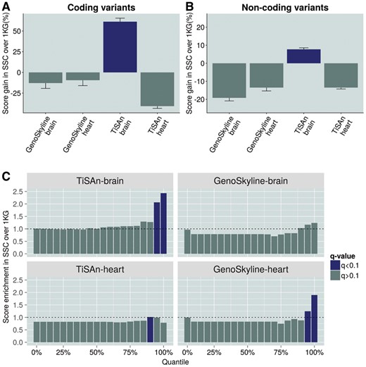
Brain-related functional enrichment in a case-control setting. Comparison of SSC variants with 1KG variants. Coding variants (A) and non-coding variants (B). Both brain and heart models for TiSAn and GenoSkyline were evaluated. (C) Functional score enrichment in SSC variants compared to 1KG variants. After sorting SSC and 1KG variants based on their score, we compute cumulative enrichment for each 5 percentile. Blue bars correspond to significant difference between SSC and 1KG, using the χ² test (FDR adjusted q-value < 0.1) (Color version of this figure is available at Bioinformatics online.)

3.3.2 Case-control variants filtering with brain-specific annotation

Next, we ranked and binned variants according to their tissue-specific scores (i.e. TiSAn or GenoSkyline) and calculated the enrichment of SSC deleterious variants in each bin, compared to deleterious 1KG variants. Because the SSC is a neurodevelopmental cohort, we expected to see over-representation of SSC variants in the most confidently called brain-related genomic regions. Indeed, significant enrichment of SSC variants was observed in the top quantiles for TiSAn-brain but also, unexpectedly, for GenoSkyline-Heart models (Fig. 3C). Surprisingly, the GenoSkyline-heart model reported a more pronounced enrichment than the corresponding brain model, suggesting a potential lack of tissue specificity for GenoSkyline. TiSAn-brain achieved the highest enrichment by ranking 2.5 times more SSC variants in the top 5% than 1KG variants.

3.3.3 Autism and calcium channel genes

An autism-related calcium voltage-gated channel gene, CACNA1C (Kabir et al., 2017), was the gene with the highest TiSAn-brain score enrichment in SSC data, suggesting that deleterious variants at this locus are likely to affect brain function. In particular, we identified 116 non-coding deleterious variants (see Section 2 for CADD thresholds) in CTCF (Prickett et al., 2013) transcription factor binding sites proximal to CACNA1C in the SSC data, while none were found in the unaffected population. Mutations in the same region also hit non-coding RNAs (ncRNAs) more frequently in the SSC population than in the control population (Fisher’s exact test, $P<2\times {10}^{-16})$⁠. Interestingly, five of these ncRNAs (Supplementary Table S8) were found in LD with loci associated with autism and Tourette’s syndrome (Ning et al., 2014).

3.4 Heart-related signal prioritization in CAD

3.4.1 Genome-wide association strength and annotation score

Current approaches to GWAS analysis rely mostly on association strength (e.g. P-value) to prioritize candidate regions. These variants often belong to large LD blocks, making it difficult to decipher the causal genetic mechanism. Here, we apply TiSAn to the Coronary Artery Disease CARDIoGRAM consortium GWAS meta-analysis (Nikpay et al., 2015), and demonstrate that the TiSAn-heart score is significantly higher among the most associated variants [Fig. 4A, (Student t-test, $P<2\times {10}^{-16}$⁠)]. Furthermore, the top 100 SNPs (according to their P-value) with a non-zero TiSAn were all found in LD with genomic regions strongly associated with CAD, demonstrating TiSAn high sensitivity. In this analysis, no significant enrichment was observed for GenoSkyline-heart (Wilcoxon signed-rank test, P = 0.12) or brain models (Fig. 4B).

Fig. 4.

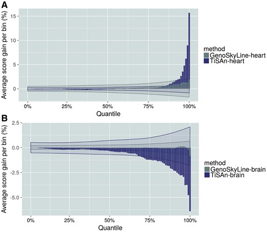
Genome-wide association signal prioritization for coronary artery disease. Genetic variants were binned by percentiles, based on their association P-values. In each of these bins, we report average functional scores for heart models (A), and brain models (B) (blue: TiSAn, gray: GenoSkyline). Shaded areas represent confidence interval for the corresponding method, after GWAS P-value random permutations (Color version of this figure is available at Bioinformatics online.)

3.4.2 Reduction of multiple hypothesis burden in GWAS

We filtered tissue-relevant genotyped variants before the GWAS analysis, using the TiSAn-heart model, so that only heart-related variants would be considered in the correction for multiple testing (herein, Bonferroni correction). In the case of CAD-GWAS, this reduced the number of SNPs considered by 75% and narrowed significant loci by 20% on average (paired Student’s t-test, P = 0.019). Furthermore, the overall enrichment in transcription factor binding sites (TFBS) among significant loci was conserved between the original and TiSAn-filtered sets (χ² test, P = 0.51), suggesting that the regulatory content was preserved after the filtering step (a further analysis of TFBS, provided in the Supplementary Material, suggests that TiSAn can reveal which TFs have important functional roles in specific tissues). Reducing the number of tested variants directly recalibrated the multiple-testing correction threshold used to determine significant loci from $5\times {10}^{-8}$ to $1.6\times {10}^{-7}$⁠. Herein, 91 new loci were found significantly associated with CAD, and these show a significant enrichment in EBF1 TFBS (Fisher’s exact test, $P=3.2\times {10}^{-6}$⁠). EBF1 is a transcription factor that has been previously linked to obesity, diabetes, and cardiovascular disease (Singh et al., 2015).

A similar analysis, using TiSAn-brain, also resulted in a substantial reduction of CAD-GWAS SNPs tested (90.2% reduction). However, consistent with proper tissue specificity, the fraction tested in this case was comparatively depleted for newly significant loci (18 additional loci for TiSAn-brain filtering, versus 90 additional loci for TiSAn-heart, $P<2.2\times {10}^{-16}$⁠, χ² test). We emphasize again that these 90 additional loci were not included in, or dependent on, the training set used for TiSAn-heart. This result supports the good generalization of the model.

4 Discussion

Integrative approaches like TiSAn hold great promise for helping genomics researchers narrow massive lists of variants to focus on those that are most relevant to the tissue or disease at hand. Few such tools currently exist, however, with most development efforts focusing on improving estimators of general (and not tissue-specific) deleteriousness (Capriotti and Fariselli, 2017). GenoSkyLine, a recently developed tool that utilizes genome-scale tissue-specific epigenetic data, allowed us to benchmark TiSAn and demonstrate its effectiveness in prioritizing genetic variants that are most likely to play a role in the tissue-specific disease processes under consideration. Specifically, we showed that individuals with elevated risk for autism (i.e. probands and their family members) had more deleterious WGS variants that were predicted to be brain relevant (by TiSAn-brain) than controls. At the same time, we were unable to show such differences in regions identified as brain-relevant by GenoSkyLine. Additionally, no difference between cases and controls was observed in TiSAn-heart score, demonstrating its specificity. We showed that strongly associated GWAS hits in a study of CAD have a significantly higher TiSAn-heart signal than non-associated SNPs, supporting our method’s ability to correctly prioritize tissue-specific variants. Again, we were unable to observe this difference using the GenoSkyLine score for cardiovascular tissue. We also demonstrated the practical advantages of reducing GWAS multiple testing burden by pre-filtering SNPs on the basis of their estimated tissue relevance. In each of these analyses, TiSAn showed an ability to correctly prioritize variants according to tissue-specific action, while GenoSkyLine, the current state-of-the-art for this application, was unable to do so. TiSAn thus represents an important development towards leveraging the massive amount of underutilized information (i.e. non-coding variation) coming from WGS studies.

Several technical points related to the development of TiSAn are worth mentioning. Perhaps most importantly, we demonstrated that combining additional data sources gives TiSAn a higher sensitivity compared to approaches that rely solely on epigenetic data. Consequently, depending on the use case, it may be worthwhile to take advantage of unique data sources that are available only for a tissue of interest, rather than only those that are available in a wide variety of tissues. Second, a comparison between multiple machine learning algorithms (Supplementary Table S5) led us to use random forests, known to better handle non-linearity and correlation between variables. Recently, deep learning has been evaluated in the context of variation effects on chromatin (Zhou and Troyanskaya, 2015), and future analyses will investigate the impact of using this algorithmic framework. Another issue is that supervised learning requires genomic positions with accurate class labels, in this case, known to be either associated with disease in a given tissue or not. However, for most of the available data, such a ‘gold standard’ label does not exist, especially for positive association with a tissue-specific trait. Imbalance-aware machine learning (Schubach et al., 2017) could be a solution to efficiently train predictive models in the case of underrepresented classes. Finally, we developed TiSAn to serve researchers with a particular focus on a single tissue by improving performance, perhaps at the expense of broad tissue coverage. Researchers interested in other tissues beyond brain or heart can derive their own functional annotation for a selected tissue of interest, and we have provided thorough documentation and software tools, including tutorials, on how to use TiSAn in typical genome informatics workflows.

Acknowledgements

We are grateful to all of the families at the participating Simons Simplex Collection (SSC) sites, as well as the principal investigators (A. Beaudet, R. Bernier, J. Constantino, E. Cook, E. Fombonne, D. Geschwind, R. Goin-Kochel, E. Hanson, D. Grice, A. Klin, D. Ledbetter, C. Lord, C. Martin, D. Martin, R. Maxim, J. Miles, O. Ousley, K. Pelphrey, B. Peterson, J. Piggot, C. Saulnier, M. State, W. Stone, J. Sutcliffe, C. Walsh, Z. Warren and E. Wijsman). Approved researchers can obtain the SSC population dataset described in this study by applying at http://sfari.org/resources/sfari-base. Data on CAD have been contributed by CARDIoGRAMplusC4D investigators and have been downloaded from www.cardiogramplusc4d.org. We also thank Tanner Koomar for editorial assistance with the manuscript.

Funding

This work was supported by the National Institutes of Health [MH105527 and DC014489 to J.J.M.].

Conflict of Interest: none declared.