Automatic selection of verification tools for efficient analysis of biochemical models

Abstract

Motivation

Formal verification is a computational approach that checks system correctness (in relation to a desired functionality). It has been widely used in engineering applications to verify that systems work correctly. Model checking, an algorithmic approach to verification, looks at whether a system model satisfies its requirements specification. This approach has been applied to a large number of models in systems and synthetic biology as well as in systems medicine. Model checking is, however, computationally very expensive, and is not scalable to large models and systems. Consequently, statistical model checking (SMC), which relaxes some of the constraints of model checking, has been introduced to address this drawback. Several SMC tools have been developed; however, the performance of each tool significantly varies according to the system model in question and the type of requirements being verified. This makes it hard to know, a priori, which one to use for a given model and requirement, as choosing the most efficient tool for any biological application requires a significant degree of computational expertise, not usually available in biology labs. The objective of this article is to introduce a method and provide a tool leading to the automatic selection of the most appropriate model checker for the system of interest.

Results

We provide a system that can automatically predict the fastest model checking tool for a given biological model. Our results show that one can make predictions of high confidence, with over 90% accuracy. This implies significant performance gain in verification time and substantially reduces the ‘usability barrier’ enabling biologists to have access to this powerful computational technology.

Availability and implementation

SMC Predictor tool is available at http://www.smcpredictor.com.

Supplementary information

Supplementary data are available at Bioinformatics online.

1 Introduction

Machine-executable mathematical and computational models of biological systems have been developed to help understand their spatial and temporal behaviours (Fisher and Henzinger, 2007). The executable nature of these models enables the design of in silico experiments, which are generally faster, cheaper and more reproducible than the analogous wet-lab experiments. The success of computational models depends crucially on two aspects: (i) the accuracy and capability to predict in vivo (or in vitro) experiments; and (ii) whether or not the methods used to validate the models can scale efficiently to handle large problem instances while maintaining the precision of the results obtained. This article deals with the latter.

Simulation and model checking (Clarke et al., 1999) are two powerful techniques used for analysing computational models. Each has its own advantages and disadvantages. Simulation works by executing the model repeatedly, and analysing the result. Each run of the system can be performed relatively quickly, but—especially in large, non-deterministic models—it is generally not possible to guarantee that every single computation path is executed. In contrast, model checking, which is an algorithmic formal verification technique, works by representing desirable properties of the model using formal mathematical logic, and then verifying whether the model satisfies the corresponding formal specification. This involves checking the model’s entire state space exhaustively by analysing all possible system trajectories. Thus, compared with simulation, model checking allows discovering more novel knowledge about system properties albeit at the expense of increased computational cost.

Model checking has been extensively used for decades in computer science and engineering in the verification of various systems, e.g. concurrent (Alur et al., 2000) and distributed systems (Norman, 2004), multi-agent systems (Konur et al., 2013), pervasive systems (Konur et al., 2014b) and swarm robotics (Konur et al., 2012), to mention just a few. Due to its novel approach to extracting information about system behaviour, it has been also applied in the analysis of biological systems and biochemical networks. Recently, it has been applied to the analysis of various systems- and synthetic-biological systems, including the ERK/MAPK pathway (Heiner et al., 2008), FGF signalling pathway (Heath et al., 2008), cell cycle in eukaryotes (Romero-Campero et al., 2006), EGFR pathway (Eker et al., 2002), T-cell receptor signalling pathway (Clarke et al., 2008), cell cycle control (Calzone et al., 2006) and genetic Boolean gates (Sanassy et al., 2014; Konur et al., 2014a).

Although model checking has been proven to be a useful method in system analysis, the very well-known state-space explosion problem associated with large non-deterministic systems (as a result of exhaustive analysis using mathematical and numerical methods) has prevented it being applied to large systems. Statistical model checking (SMC) (Younes and Simmons, 2002) has been introduced to alleviate the state-explosion problem issue by replacing mathematical and numerical analysis with a simulation approach (where a number of system trajectories are considered instead of exhaustive analysis), which is computationally less demanding. That is, SMC combines simulation and model checking, thereby leveraging the speed of simulation with the comprehensive analytical capacity of model checking. The greatly reduced number of executions enables verification of larger models at far lower computational cost, albeit by introducing a small amount of uncertainty.

The success of SMC has prompted researchers to implement a number of SMC tools, e.g. probabilistic and symbolic model checker (PRISM) (Hinton et al., 2006), Ymer (Younes, 2005), Markov reward model checker (MRMC) (Katoen et al., 2009), Monte Carlo Model Checker (MC2) (Donaldson and Gilbert, 2008) and PLASMA-Lab (Boyer et al., 2013). In order to facilitate the model checking process, SMC tools have also been employed as third party tools in a number of integrated software suites, such as SMBioNet (Khalis et al., 2009), Biocham (Faeder et al., 2009), Bio-PEPA Eclipse Workbench (Ciocchetta and Hillston, 2009), genetic network analyser (Batt et al., 2012), kPWorkbench (Bakir et al., 2014; Dragomir et al., 2014) and Infobiotics Workbench (Blakes et al., 2011, 2014).

Despite its clear computational advantages, SMC also has drawbacks. Although a large variety of tools have been developed, the performance of each tool significantly varies according to the topological features and characteristics of the underlying network of a given model (e.g. number of vertices and edges, graph density, graph degree etc.) and the type of system requirements/properties being verified. The model features and characteristics can affect the verification performance hugely (as well as simulation performance, as shown in Sanassy et al., 2015); in particular, verification of models with more complex network structures tend to be more challenging. As we showed in a recent work (Bakir et al., 2017), the type of biological property (i.e. requirement) can also significantly affect the verification time, as each property type can involve different computational processes on the network working at different levels of complexity (e.g. searching some nodes, or all nodes etc.).

This makes it hard to know—a priori—which model checking tool is the most efficient one for a given biological model and requirement, as this requires a significant degree of computational expertise, not usually available in biology labs.

Thus, while the availability of multiple variants of these tools and algorithms can allow considerable flexibility and fine-tuned control over the analysis of specific models, it is very difficult for non-expert users to acquire the knowledge needed to identify clearly which tools are the most appropriate. It is therefore important to have a way of identifying and using the fastest SMC tool for a given model and property.

The objective of this article is to introduce a method and provide a tool leading to the automatic selection of the most appropriate model checker for the system of interest. This will not only significantly reduce the total time and effort requested by the use of the model checking tools, but will also enable more precise verification of complex models while keeping the verification time tractable. In consequence, a deeper understanding of biological system dynamics will be acquired in a significantly improved time scale and with better performances.

1.1 Contributions

In this work, we have introduced a novel approach that combines various aspects of computer science, including formal verification, stochastic simulation algorithms (SSAs) and machine learning to improve computational analysis—via model checking—in systems and synthetic biology by addressing performance related issues through novel computing solutions. To this end, we have developed a systematic and effective methodology: We have first identified some model features that represent topological and graph theoretic characteristics of the model. We have benchmarked the five of the most commonly used SMC tools by verifying 675 biological models against various commonly used biological requirements (so called patterns). Using the identified model features, we have then utilised several machine learning techniques on the data obtained to train efficient and accurate classifiers. We have demonstrated that our approach can predict the fastest SMC tool with over 90% accuracy. This implies a huge performance gain compared with the random selection of tools, as choosing the most efficient model checker will result in significantly less verification time. We have implemented our approach and developed a software system, SMC Predictor, that predicts the fastest SMC tool based on a given biomodel and biological property.

To the best of our knowledge, this is the first paper that addresses the performance related issues of SMC tools in connection with model structure and the property.

2 Materials and methods

2.1 SMC tools

In this section, we briefly describe the five widely used SMC tools considered in our experimental analysis: PRISM (Hinton et al., 2006), Ymer (Younes, 2005), MRMC (Katoen et al., 2009), MC2 (Donaldson and Gilbert, 2008) and PLASMA-Lab (Boyer et al., 2013). These tools have been used for analysing a wide range of systems, including computer, network and biological systems. The applicability of these SMC tools to a broad range of biological systems has been intensively investigated (Jansen et al., 2008; Bakir et al., 2017; Boyer et al., 2013; Donaldson and Gilbert, 2008; Zuliani, 2015).

PRISM is a popular and well-maintained probabilistic model checker tool (Hinton et al., 2006). PRISM implements both probabilistic model checking based on numerical techniques with exhaustive analysis of the model and SMC using an internal discrete-event simulation engine (Kwiatkowska et al., 2007). PLASMA-Lab is another SMC for analysing stochastic systems (Boyer et al., 2013). In addition to its internal simulator, it also provides a plugin mechanism to users, allowing them to integrate custom simulators into the PLASMA-Lab platform. Ymer is one of the first tools that implemented SMC algorithms—its ability to parallelise the execution of simulation runs makes it a relatively fast tool (Younes, 2005). MRMC is another tool which can support both numeric and SMC of probabilistic systems. Finally, MC2 enables SMC over simulation paths. Although this tool does not have an internal simulator, it permits using simulation paths of external simulators (Donaldson and Gilbert, 2008).

2.2 Property patterns

Model checking uses temporal logics (Clarke et al., 1999) to specify desired system properties and requirements. But this is a very tedious task, because writing such formal specifications requires a very good understanding of formal languages. In order to facilitate the property specification process for non-experts, various frequently used property types (patterns) have been identified in previous studies (Dwyer et al., 1999; Grunske, 2008; Monteiro et al., 2008); and we have done likewise for patterns that are particularly appropriate for biological models (Konur, 2014; Gheorghe et al., 2015; Konur and Gheorghe, 2015). These patterns are commonly recurring properties that one may want to check in a modelled system.

We have identified 11 popular property patterns that are used in our experimental settings. The precise definitions of the property patterns and the model checking tools supporting them are provided using a systems level model of P.aeruginosa quorum sensing as an example (see Supplementary Section 2).

2.3 Models

In order to identify the performance of SMC tools, we have verified instances of the 11 patterns on 675 up-to-date biological models taken from the BioModels database (http://www.ebi.ac.uk/) in SBML format, a data exchange standard. In order to focus on the model structure analysis, we have fixed stochastic rate constants of all reactions to 1.0 and the amounts of all species to 100 (in previous work (Sanassy et al., 2015), 380 of these models were considered in a similar fashion to predict performance of simulation tools). The models tested ranged in size from 2 species and 1 reaction, to 2631 species and 2824 reactions. The distribution of model sizes can be found in Supplementary Section 4.2 (Fig. 1).

Fig. 1.

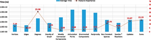
Computational time and feature importance. Average computational time and feature importance associated with model topological properties

In this article, we focus on predicting the time performance of a set of available model checkers in order to save the end-user computational expense. In previous work Sanassy et al. (2015), we have shown that we can reliably focus on the model structure only to make such performance prediction when trying to decide on the fastest simulation engine. That is, model parameters could be safely ignored while still being able to robustly predict the best simulator to use. More recently, it has been demonstrated that a similar approach (namely focussing on structure and ignoring parameters) was sufficient to predict the outcome of long stochastic chemical simulations Markovitch and Krasnogor (2018). Thus, we follow a similar approach here and focus solely on model structure and ignore model parameters for the purpose of predicting the speed at which different model checkers verify system level models.

We have also run an additional experiment to demonstrate that keeping the model parameters as they are does not affect the prediction accuracy. The details can be found in Supplementary Section 4.4

2.4 Prediction

In order to train the classifiers, we utilised several different machine learning algorithms implemented in the scikit-learn library (Pedregosa et al., 2011). We have compared seven methods; five of them are powerful and widely used algorithms, namely, support vector machine classifier (SVM) (Chang and Lin, 2011), logistic regression (LR) (Yu et al., 2011), K-nearest neighbour classifier (KNN) (Mucherino et al., 2009), extremely randomized trees (ERT) (Geurts et al. 2006) and random forests (RFs) (Breiman, 2001) and two of the classifiers are for baseline predictions, namely, Random Dummy (RD) and Stratified Dummy (SD). We used 10-fold cross-validation for training and testing the classifiers. An alternative validation method is provided in Supplementary Section 4.3.

2.5 SMC predictor tool

We have developed a software system, SMC Predictor, which accepts biomodels written in SBML and property patterns as input, and returns the prediction of which stochastic model checker the user should use, giving preference to time required for the verification process. The classifiers predict the fastest SMC tool for each model and property pattern. The software system architecture is presented in Supplementary Section 5.

The experimental data and the SMC Predictor tool are available at http://www.smcpredictor.com.

3 Results and discussion

In this section, we present the results of benchmarks with the five of the most commonly used SMC tools by verifying 675 biological models against various commonly used biological requirements (patterns) and then analyse the accuracy of predicting the fastest SMC tool by using classifiers, based on machine learning techniques involving identified model features and trained on the data obtained. Supplementary Section 4.1 describes the system configuration and the current versions of the SMC tools used in our experiments.

We start by presenting experiments showing the average computational time required for various model features and the impact these features have on the prediction accuracy.

3.1 Feature selection

Topological and graph-theoretic features of the underlying network of a model (e.g. number of vertices and edges, graph density, graph degree etc.) significantly affect the simulation time of SSAs. These features have been used to predict the performance of SSAs (Sanassy et al., 2015), although a restricted number of graph features was used to reduce the complexity of the prediction process, as the computation of some of the features which generally require graph construction is computationally demanding. This resulted in a relatively low accuracy rate, 63%.

The performance of stochastic model checking depends primarily on such model features as well as the property type being queried (Bakir et al., 2017). In our work, we aim to increase the predictive accuracy without compromising on computation time. In addition to the graph topological features, we have therefore considered new features which mostly do not require graph construction (e.g. number of species whose values can change; number of species multiplied by number of reactions; min, max and mean number of variable changes; total number of all incoming and outgoing edges). The graph-related features and our newly introduced (non-graph related) ones are described in Supplementary Section 3.

The bar chart in Figure 1 shows the average computational time (in nanoseconds) required when using each topological feature. In order to identify which of the properties are most important for our purposes, we have conducted feature selection analysis using a feature importance algorithm based on ERTs (Geurts et al., 2006; Louppe et al., 2013). The data points on the line graph in Figure 1 show the ‘percentage importance’ of each feature. The results show that graph-theoretic features such as reciprocity, weakly connected components, biconnected components and articulation points are computationally expensive but actually contribute less to the predictive power than the computationally less expensive features.

In addition to the above experiments we have evaluated the prediction accuracy of the method described in Sanassy et al. (2015) in the context of the extended set of features. Better results have been obtained when non-graph-related features are considered and computationally expensive graph-theoretic ones are removed (details in Supplementary Section 4.2).

Based on these results we have considered for the final features set those that give better prediction accuracy with a reasonable computational time.

3.2 Performance benchmarking of SMC tools

We have benchmarked the performance of 5 SMC tools using 675 biomodels obtained from the EBI database (http://www.ebi.ac.uk/) against 11 property patterns. This is a significant extension of our previous work (Bakir et al., 2017), where we only considered a small subset of models and property patterns with a significantly less number of experiments. Since all models are available in the SBML format, we have developed a tool translating the SBML model into the syntax that these SMC tools accept as input. The tool also translates the property patterns into the formal specification languages of the model checkers.

For each test 500 simulation traces were generated and 5000 steps per trace were executed. Each test was repeated three times and the average time considered. The elapsed time for each run includes the time required for model parsing, simulation and verification, and where one tool depends on the use of another one then the execution time of the auxiliary tool is included in the total execution time.

Table 1 summarises our experimental results. PLASMA-Lab could verify all models; MC2 could verify most models for all property patterns, except Precedes. MC2 failed to verify only a few models within the available time. Ymer could also verify most of the models, but could not handle and repeatedly crashed for 31 large models. PRISM’s capacity for verification depends on the pattern type; for example, it could verify only 364 models against the Eventually pattern but it could verify almost all models, 672, for the Precedes pattern. The reason is that PRISM requires a greater simulation depth for unbounded property verification to have a reliable approximation. MRMC could verify fewer models than the other SMCs for all property patterns, because it relies on PRISM for transition matrix generation. However, for medium sized and large models PRISM failed to build and export the transition matrices—we believe this was due to a CU Decision Diagram library crash.

Table 1.

The number of models verified against different property patterns

	PRISM		PLASMA-Lab		Ymer		MRMC		MC2
Patterns	Verif.	Fast.	Verif.	Fast.	Verif.	Fast.	Verif.	Fast.	Verif.	Fast.
Eventually	364	18	675	248	644	402	116	3	668	4
Always	480	80	675	132	644	457	118	2	668	4
Follows	N/A	N/A	675	575	N/A	N/A	116	39	664	61
Precedes	672	170	675	18	644	486	113	0	664	1
Never	542	103	675	147	644	422	116	1	668	2
Steady state	N/A	N/A	675	579	N/A	N/A	80	30	668	66
Until	592	125	675	82	644	465	112	0	664	3
Infinitely often	N/A	N/A	675	604	N/A	N/A	N/A	N/A	668	71
Next	658	581	675	17	N/A	N/A	118	36	675	41
Release	622	151	675	49	644	472	111	0	664	3
Weak until	591	126	675	82	644	465	112	0	664	2

Note: Columns labelled Verif. show the number of models verified by each tool. Columns labelled Fast. show for how many models the corresponding tool was the fastest. N/A, not applicable, means the corresponding pattern is not supported by the tool.

Figure 2 illustrates the relation between the fastest tool and model size. Ymer is the fastest tool for most of the models (for the supported property patterns), however, as Figure 2 shows, it was generally the fastest for relatively small sized models. PRISM and PLASMA-Lab are generally the fastest tools for medium to large sized models. It may be observed that their performances vary across different property patterns. MRMC and MC2 are the fastest tools for fewer models and they perform best only for small sized models. They do slightly better for the Follows, Steady State and Infinitely Often patterns where they compete with fewer tools.

Fig. 2.

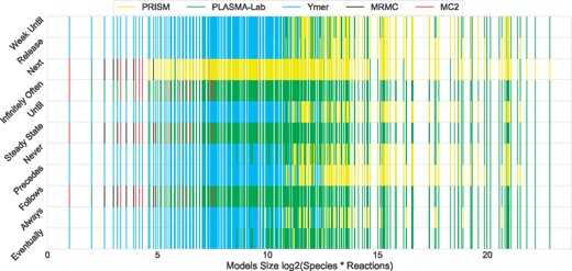
Fastest SMC tools verifying each model against each property pattern. The X-axis represents logarithmic scale of model size; the Y-axis shows the property patterns. For each model a one-unit vertical line is drawn against each pattern. The line’s colour shows the fastest SMC

Figure 3 illustrates the verification time for each tool with respect to model size, providing complementary information to what is in Table 1 and Figure 2. The figure shows the tool performance comparison for two patterns. The results for all patterns are presented in Supplementary Section 4.5. Generally speaking, MC2 and MRMC require more time for verification; hence they are less efficient compared with the other tools. In particular, MRMC can verify very few models and its verification time increases exponentially for the larger models. The verification time for Ymer increases almost linearly, i.e. it is fast for small models, but the verification time constantly increases when the model size increases. PLASMA-Lab displays an exponential growth for small size models but it gets more efficient for large size models. Like PLASMA-Lab, PRISM generally is not the fastest option for small-sized models whereas it can perform better for larger models.

Fig. 3.

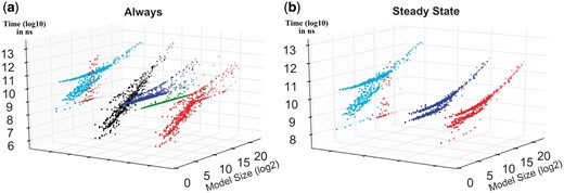
Performance comparison. For each property pattern, each tool performance is compared against the best performance. Here, X-axes represent the model size (species × reactions) in logarithmic scale (log₂), Y-axes show the relative performance of each SMC tool in comparison with the fastest one, and Z-axes show (log₁₀ scale) the consumed time in nanoseconds

These results show that the performance of the model checking tools significantly changes based on models and property patterns, which makes it extremely difficult to predict the best tool without the assistance of an automated system.

3.3 Automating SMC tool prediction

We have used five machine learning techniques and two random selection algorithms, RD and SD, for predicting the fastest SMC tool. The random selection algorithms were used for comparing the success rate of each algorithm with random prediction. The RD classifier ‘guesses’ the SMC tool blindly, that is, with uniform probability 1/5 it picks one of the five verification tools at random, whereas the SD classifier knows the distribution of the fastest SMC tools. The RD classifier acts as a proxy for the behaviour of the researchers who do not know much about model checking tools, while SD can be considered as mirroring the behaviour of experienced verification researchers who know the patterns supported by each tool and the fastest tools distribution, but do not know which is the best tool for a specific property to be checked on a specific model. The remaining five methods are: SVM classifier (Chang and Lin, 2011); LR (Yu et al., 2011); KNN classifier (Mucherino et al., 2009); and two types of ensemble methods, namely, ERT (Geurts et al., 2006) and RFs (Breiman, 2001) (despite their names these are not random classifiers, but ensemble classifiers). We used the scikit-learn library (Pedregosa et al., 2011) implementation of these classifiers in our experiments.

We have considered three different accuracy scores in our experiments. The first score, ‘S1’, is the percentage of correct estimation of the fastest SMC tool with the 10-fold cross-validation. The second score, ‘S2’, is calculated by considering a threshold bound to assessing a correct prediction, namely, whenever the relative time difference between the actual fastest SMC tool and the predicted fastest SMC tool is not >10% of the actual fastest SMC tool time, then the prediction is considered correct. For the third score, ‘S3’, the order of the fastest SMC tools is used and if the predicted SMC tool is the second fastest tool, then it is regarded as a correct prediction.

The experimental results with first score (S1) of each classifier for different property patterns are shown in Figure 4 and their accuracy values are tabulated in Table 2. The success rates were all higher than for random classifiers. ERT was the most frequent winner, as it had best predictive accuracy for six patterns (for Infinitely Often, ERT and LR have the same highest accuracy, 95%), whereas the SVM classifier was the second best winner with highest predictive accuracy for five patterns. ERT and SVM are hereinafter referred to as the best classifiers. The prediction accuracies of the best classifiers were over 90% for all pattern types.

Table 2.

Accuracy values using first score (S1)

	SVM	ERT	RF	LR	KNN	SD	RD	P-value
Eventually	92.4%	92.2%	91.6%	92.0%	88.8%	47.7%	12.4%	3.4e-09
Always	88.9%	90.5%	90.1%	85.9%	84.7%	53.4%	16.3%	8.1e-09
Follows	95.0%	93.6%	93.9%	92.4%	92.6%	70.5%	29.1%	3.5e-08
Precedes	95.4%	97.2%	97.0%	93.5%	94.4%	63.3%	27.4%	1.1e-09
Never	88.5%	91.0%	89.8%	85.6%	85.2%	48.8%	19.1%	3.5e-09
Steady state	94.2%	93.2%	92.6%	93.0%	92.7%	70.7%	29.6%	1.1e-07
Until	91.0%	92.8%	92.2%	87.8%	88.0%	54.7%	28.7%	4.5e-08
Infinitely often	91.6%	95.0%	94.7%	95.0%	93.6%	81.5%	61.2%	7.4e-09
Next	94.3%	93.5%	92.9%	92.6%	93.5%	72.9%	36.9%	1.9e-07
Release	94.2%	93.8%	93.1%	89.8%	91.3%	58.8%	28.4%	1.9e-08
Weak until	90.8%	92.3%	91.7%	88.8%	87.1%	57.4%	27.3%	2.4e-08
P-value	8.0e-08	2.9e-04	1.1e-05	1.7e-09	2.1e-09	2.4e-14	4.6e-13

Fig. 4.

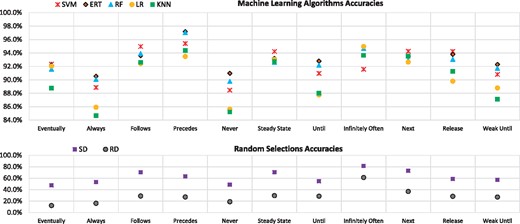
Predictive accuracies. Accuracies (S1) for the fastest SMC prediction with different algorithms

We have measured the P-values of each classifier across different property patterns, by comparing the accuracy scores of cross-validation of each classifier using the Friedman test (Friedman, 1940) provided with the Python SciPy library (http://scikit-learn.org). Table 2 provides both row- and column-wise P-values. The column-wise P-values indicate that, a given classifier (e.g. SVM) views the predictive accuracies of different patterns with statistically significant differences (i.e. low P-values). So, it would not be recommended to use just one classifier for all pattern types. The row-wise P-values indicate that, for a given pattern (e.g. ‘Eventually’) the prediction accuracy might be more readily done via different classifiers with statistically significant differences. That is, the low P-values suggest that different methods have statistically different performances.

Table 3 shows the experimental results using the other score settings. The accuracy of ‘S2’ experiments is not much higher than for ‘S1’, which considered only the actual fastest tool prediction as correct, but the accuracy of ‘S3’ is significantly higher because it ‘lumps together’ the fastest and second fastest tools, but the time differences between the second best and the actual best tool can be orders of magnitude, i.e. much more than 10-fold. For the Follows, Steady State and Infinitely Often patterns, the accuracies of SD and RD are relatively better under these more relaxed scoring approaches, because there are fewer tools which support these patterns; hence they have higher chances of correct prediction. Similar to Table 2, Table 3 provides both row- and column-wise P-values. The row-wise P-values indicate that there are statistically significant differences when using the same classifier for different patterns. The column-wise P-values indicate that for a given pattern the prediction accuracy varies for different classifiers with statistically significant differences.

Table 3.

Predictive accuracy with different score settings

		Eventually	Always	Follows	Precedes	Never	Steady state	Until	Infinitely often	Next	Release	Weak until	P-value
SVM	S2	94.1%	91.1%	95.7%	96.6%	89.8%	95.3%	91.9%	92.3%	95.4%	95.4%	92.6%	1.9e-07
	S3	98.7%	96.4%	99.1%	98.1%	94.4%	99.3%	95.1%	100.0%	97.2%	97.9%	96.7%	2.8e-10
ERT	S2	93.7%	92.2%	94.8%	98.1%	92.7%	94.1%	94.3%	95.9%	94.7%	95.3%	93.9%	5.6e-04
	S3	98.4%	96.9%	98.5%	99.6%	96.1%	99.0%	97.8%	100.0%	96.6%	97.8%	97.6%	2.8e-07
RF	S2	93.4%	91.8%	95.0%	98.7%	91.5%	93.6%	93.6%	95.4%	94.3%	95.4%	93.2%	2.6e-04
	S3	99.0%	97.0%	99.3%	99.9%	96.0%	99.1%	97.3%	100.0%	96.3%	97.6%	97.0%	2.8e-09
LR	S2	93.8%	88.6%	93.6%	95.1%	87.5%	94.2%	90.0%	95.9%	93.8%	91.9%	90.4%	3.2e-08
	S3	99.0%	95.4%	99.1%	97.3%	93.8%	99.7%	95.1%	100.0%	96.1%	95.1%	95.1%	4.9e-11
KNN	S2	90.2%	87.5%	93.6%	96.0%	87.7%	93.6%	90.5%	94.5%	94.7%	92.8%	89.6%	2.6e-08
	S3	96.7%	94.5%	98.1%	98.7%	93.2%	98.5%	95.4%	100.0%	96.0%	95.1%	94.4%	1.3e-09
SD	S2	49.3%	55.7%	70.5%	64.9%	52.3%	71.4%	56.9%	82.4%	78.1%	60.7%	59.4%	3.3e-14
	S3	71.7%	71.9%	90.5%	75.0%	72.4%	90.4%	70.8%	100.0%	86.8%	72.4%	74.8%	9.9e-13
RD	S2	13.6%	17.3%	30.5%	31.8%	19.7%	30.7%	30.9%	61.5%	38.4%	31.7%	28.9%	1.4e-12
	S3	32.9%	35.0%	65.0%	49.5%	39.4%	64.3%	48.0%	99.3%	56.0%	47.6%	47.9%	8.6e-15
P-value	S2	3.3e-09	2.8e-08	3.5e-08	2.4e-09	3.1e-09	8.3e-08	1.1e-08	5.0e-09	1.8e-07	2.1e-08	7.0e-09
	S3	2.2e-09	5.3e-08	1.6e-08	5.4e-10	2.4e-08	2.6e-08	7.3e-09	5.2e-04	2.4e-07	2.1e-08	1.1e-08

3.4 Performance gain and loss

In this section, for each property pattern, we have assessed the performance gain and loss for the best classifiers and the random classifiers. The performance gain is the time difference between the verification time of the tools predicted by the best classifiers and the random classifiers.

Figure 5 shows the total time required to verify all models with the actual fastest SMC tools, the best classifier predictions and the random classifier predictions. The performance gain between the best classifiers and the SD classifier is minimum 63 min for Infinitely Often, maximum 3002 min for Always, and average 1848 mins for all patterns. The time difference between the best classifiers and RD is even larger: minimum 528 min, maximum 12 506 min and average 6109 min for all patterns. The results show that using the best classifier predictions a significant amount of time can be saved—up to 208 h!

Fig. 5.

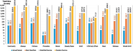
Total time consumed for verifying all models

Generally, the outcomes of mispredictions can be as important as correct predictions. In this regard, we have measured the performance loss caused by inaccurate predictions. Figure 6 shows the performance loss, i.e. time difference between the total verification time using the actual fastest SMC tools and the total verification time using the predicted SMC tools. The performance loss for the best classifier is minimum 0.3 min for Precedes, maximum 885 min for Next, and average 318 min for all patterns. Similarly, the performance loss for SD is minimum 67 min, maximum 3662 min and average 2167 min; for RD is minimum 532 min; maximum 12 567 min and average 6427 min. The results suggest the best classifiers’ performance losses are always lower than the random classifiers’ ones. More specifically SD and RD cause performance losses 7 and 20 times, respectively, higher than the best classifiers.

Fig. 6.

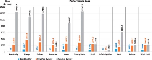
The mean performance loss when the best classifiers predict incorrectly

Finally, Table 4 provides the best, worst and predicted model checking times for a set of selected models and patterns (note that we have put a 1-h cap on the length of each experiments; the worst model checking times presented are generally > 1 h (in some cases, hours or even days)). The best times and predicted times for each pattern are mostly identical; as previously discussed the prediction accuracy is very high.

Table 4.

Best, worst and predicted model checking time (seconds) for various models and patterns

	Always			Eventually			Until
Model	Best	Worst	Predicted	Best	Worst	Predicted	Best	Worst	Predicted
1	0.09	>3600	0.09	0.25	>3600	0.25	0.08	>3600	0.08
2	0.08	>3600	0.08	0.26	>3600	0.26	0.08	>3600	0.08
3	0.07	>3600	0.07	0.14	>3600	0.14	0.08	>3600	0.08
4	0.63	>3600	0.63	1.26	>3600	1.26	0.34	>3600	0.34
5	0.67	>3600	0.67	1.30	>3600	1.30	0.34	>3600	0.34
6	0.31	>3600	0.31	0.58	>3600	0.58	0.33	>3600	0.33
7	1.49	>3600	1.49	8.63	>3600	8.63	1.49	>3600	2.14
8	1.51	>3600	1.51	6.01	>3600	6.01	2.92	>3600	5.01
9	1.54	>3600	1.54	4.29	>3600	4.29	1.50	>3600	1.50
10	121.00	>3600	121.00	195.00	>3600	195.00	3.23	>3600	3.23
11	118.00	>3600	118.00	201.00	>3600	201.00	6.24	>3600	6.24
12	64.06	>3600	64.06	385.00	>3600	385.00	3.37	>3600	3.37

The results show that (even with a one hour cap) one can achieve a significant performance gain. While a random selection might lead to hours of model checking time, using the predictor can reduce this time to milliseconds. In a typical formal analysis of a system, where several queries are used to verify desired system properties, experiments that might take hours or days to run can be reduced to minutes or even seconds.

3.5 Conclusion

In this article, we have proposed and implemented a methodology to automatically predict the most efficient SMC tool for any given model and property pattern. To do so, we first proposed a set of model features which can be used for SMC prediction. We then systematically benchmarked several model checkers by verifying 675 biological models against 11 property patterns. By utilizing several machine learning algorithms, we have generated efficient and accurate classifiers that successfully predict the fastest SMC tool with over 90% accuracy for all pattern types. We have developed software using built-in classifiers to make the prediction automatically. Finally, we have shown that by using automated prediction, a significant amount of time can be saved.

For the next stage of our work, we aim to integrate the automated fastest SMC prediction process into some of the larger biological model analysis suites, e.g. kPWorkbench (Dragomir et al., 2014) and Infobiotics Workbench (Blakes et al., 2011).

Funding

This work was supported by the Engineering and Physical Sciences Research Council [grant numbers EP/I031642/2 to S.K., M.G. and N.K. and EP/J004111/2, EP/L001489/2 and EP/N031962/1 to N.K.]; Innovate UK [grant number KTP010551 to S.K.]; the Romanian National Authority for Scientific Research (CNCS-UEFISCDI) [project number PN-III-P4-ID-PCE-2016-0210 to M.G.]; and the Turkey Ministry of Education [PhD studentship to M.E.B.].

Conflict of Interest: none declared.