LZW-Kernel: fast kernel utilizing variable length code blocks from LZW compressors for protein sequence classification

Abstract

Motivation

Bioinformatics studies often rely on similarity measures between sequence pairs, which often pose a bottleneck in large-scale sequence analysis.

Results

Here, we present a new convolutional kernel function for protein sequences called the Lempel-Ziv-Welch (LZW)-Kernel. It is based on code words identified with the LZW universal text compressor. The LZW-Kernel is an alignment-free method, it is always symmetric, is positive, always provides 1.0 for self-similarity and it can directly be used with Support Vector Machines (SVMs) in classification problems, contrary to normalized compression distance, which often violates the distance metric properties in practice and requires further techniques to be used with SVMs. The LZW-Kernel is a one-pass algorithm, which makes it particularly plausible for big data applications. Our experimental studies on remote protein homology detection and protein classification tasks reveal that the LZW-Kernel closely approaches the performance of the Local Alignment Kernel (LAK) and the SVM-pairwise method combined with Smith-Waterman (SW) scoring at a fraction of the time. Moreover, the LZW-Kernel outperforms the SVM-pairwise method when combined with Basic Local Alignment Search Tool (BLAST) scores, which indicates that the LZW code words might be a better basis for similarity measures than local alignment approximations found with BLAST. In addition, the LZW-Kernel outperforms n-gram based mismatch kernels, hidden Markov model based SAM and Fisher kernel and protein family based PSI-BLAST, among others. Further advantages include the LZW-Kernel’s reliance on a simple idea, its ease of implementation, and its high speed, three times faster than BLAST and several magnitudes faster than SW or LAK in our tests.

Availability and implementation

LZW-Kernel is implemented as a standalone C code and is a free open-source program distributed under GPLv3 license and can be downloaded from https://github.com/kfattila/LZW-Kernel.

Supplementary information

Supplementary data are available at Bioinformatics Online.

1 Introduction

Over the last two decades, two interesting alignment-free approaches have emerged for protein sequence comparison. The first one builds on the universal compressibility of sequences and is widely used for clustering (Cilibrasi and Vitanyi, 2005) or phylogeny (Li et al., 2001). The second approach aims at building novel discrete kernel functions that could directly be plugged into Support Vector Machines (SVMs) for discriminative protein sequence classification or protein homology detection (Haussler, 1999; Jaakkola et al., 1999).

The interest in normalized compression distance (NCD) methods was fostered by Ming Li et al.’s seminal paper (Li et al., 2001), in which they applied the GenCompress algorithm to estimate the distance between mitochondrial genomes. This was followed by another paper (Li et al., 2003), in which they proved that a simple sequence compressibility index is actually better than n-gram techniques. Soon, NCD appeared in various practical applications including protein sequence and structure classification (Ferragina et al., 2007; Kertész-Farkas et al., 2008a, b; Krasnogor and Pelta, 2004; Kocsor et al., 2006), language classification (Benedetto et al., 2003; Li et al., 2003), hierarchical clustering (Cilibrasi and Vitanyi, 2005; Kraskov et al., 2003), music classification (Cilibrasi et al., 2004) and clustering fetal heart rate tracings (Santos et al., 2006). The normalized compression-based distance was defined by Cilibrasi and Vitányi in (Cilibrasi and Vitanyi, 2005) as

$$\text{NCD}(x,y)=\frac{C\left(xy\right)-\min \left\{C\right(x),C(y\left)\right\}}{\max \left\{C\right(x),C(y\left)\right\}},$$

(1)

where C(x) denotes the length of a compressed string compressed by a casual text compressor such as zip. One of the most well-known text compressors is the Lempel–Ziv–Welch (LZW) compressor (Ziv and Lempel, 1977); it is widely used because it is fast and simple. It was shown that NCD is a distance metric up to an additive term $O\left(\right(\text{log}\hspace{0.17em}n)/n)$⁠, if the compressor C satisfies the following properties: Idempotency (⁠$C\left(xx\right)=C\left(x\right)$ and $C(\lambda )=0$⁠, where λ is the empty string), Symmetry (⁠$C\left(xy\right)=C\left(yx\right)$⁠), Monotonicity: (⁠$C\left(xy\right)\ge C\left(x\right)$⁠) and Distributivity: (⁠$C\left(xy\right)+C\left(z\right)\le C\left(xz\right)+C\left(yz\right)$⁠) up to an additive term $O(\text{log}\hspace{0.17em}n)$⁠, where n is the highest complexity of a string that appears in the (in)equality (Cilibrasi and Vitanyi, 2005). However, in practice, NCD violates the metric properties quite often. It was shown that it is not always symmetric and it violates the triangle inequality and the identity of indiscernibles. For more details, we refer the reader to (Kertész-Farkas et al., 2008a, b).

Kernel functions can be regarded as similarity functions which have the additional property of always being positive semi-definite [see (Berg et al., 1984)]. Kernel functions provide a plausible way to extend linear vector and scalar product-based applications to a non-linear model while preserving their computational advantages (Shawe-Taylor and Cristianini, 2004). Furthermore, kernel functions can be directly applied to non-vectorial data like strings, trees and graphs. For discrete data structures such as strings, trees, or graphs, Haussler has given a general way to construct new kernel functions, called convolutional kernels (Haussler, 1999). Basically, they convolve simpler kernel functions to obtain more complex ones. The convolutional kernel goes over all possible decompositions of input structures, which can be intractable in practice. Over the past two decades, many kernels have been developed for protein sequence classification, protein homology detection, or protein–protein interaction detection problems such as the string kernels (Lodhi et al., 2002), context tree kernels (Cuturi and Vert, 2005), mismatch kernel (MMK) (Leslie et al., 2004), spectrum kernel (Leslie et al., 2002), local alignment kernel (LAK) (Vert et al., 2004), Fisher kernel (Jaakkola et al., 1999), pairwise kernel for protein–protein interaction prediction (Vert et al., 2007) and support vector kernels (Dombi and Kertész-Farkas, 2009; Kertész-Farkas et al., 2007) in combination with SVMs.

The spectrum kernel calculates the scalar products of an n-gram representation of two sequences; however, it does so without implicitly calculating the actual large dimensional n-gram vectors. This requires O(nN) time, where N is the total length of the input. MMKs and string kernels further generalize this, as they allow a certain amount of mismatches (m) or gaps when counting the common n-mers. The MMK is relatively inexpensive for m and n values that are practical in applications and for M sequences each of length k, it has a worst-case complexity of $O\left(M^{2}k{n}^m{l}^m\right)$⁠, where l is the size of the alphabet (20 for amino acids and 4 for nucleotides). Unfortunately, MMK becomes impractical for any m > 1.

The Fisher kernel combines the rich biological information encoded into a generative hidden Markov model (HMM) with the discriminative power of the SVM algorithm. However, the training of HMMs requires lot of data and the Fisher score calculation requires the dynamic-programming based Viterbi algorithm, which is quadratic in the sequence length for profile HMMs. Thus, the Fisher kernel is computationally very expensive in practice (Leslie et al., 2004).

Sequence alignment methods, such as Smith–Waterman (SW) and Basic Local Alignment Search Tool (BLAST) are perhaps the best-performing methods for biological sequence similarity. The scoring is mainly based on the so-called substitution matrix, e.g. BLOSUM62 and gap penalties which encode rich biological knowledge, where the power of these methods comes. Unfortunately, these methods are only similarity measures, but not kernel functions; thus, they cannot be directly used with SVMs (Cristianini and Shawe-Taylor, 2000). LAK can be considered the kernelized version of SW. LAK, roughly speaking, summarizes all the local alignments contrary to SW, which simply uses the best scoring local alignment. Both methods, LAK and SW, have a polynomial time complexity $O\left(N^2\right)$ for sequences of total length N.

In this article, we introduce a new convolutional kernel function for sequence similarity measures called LZW-Kernel, which can be used with SVMs. It utilizes the LZW compressor to give the best decomposition of the input sequences x and y; therefore, the convolutional kernel does not need to iterate over all possible decompositions. Then, roughly speaking, LZW-Kernel calculates a weighted sum of the common blocks. Because the LZW compression is a single pass method, the LZW-Kernel function is also extremely fast. We note that because the LZW compression is related to the entropy of the input string, the LZW-Kernel is likely to have an information theoretic interpretation. This is the topic of one of our ongoing research.

The LZW-Kernel has more favorable characteristics than NCDs have. For instance, the normalized LZW-Kernel is always symmetric, is positive valued, always provides 1.0 for identical sequences, and it can be used directly with SVMs. In contrast, NCDs often violate the metric properties using various compressors, as was shown in our former work (Kertész-Farkas et al., 2008a, b); moreover, NCDs cannot be used with SVMs directly because they are neither positive definite kernels nor similarity functions. Overcoming these disadvantages of NCDs was our main motivation in developing LZW-Kernel. While NCD is fast, the LZW-kernel is around 30–40% faster. In addition, our experimental tests show that the LZW-Kernel provides better performance on remote protein homology detection using SVMs than NCDs using LZW compressors with the SVM-pairwise approach. These facts about LZW-kernel shows its great advantages compared to NCDs.

In the next section, we formally introduce our new convolutional kernel. In Section 3, we introduce our testing environment and describe the datasets and methods we used. This is followed by Section 4, in which we present and discuss our experimental results. Finally, we summarize our findings and conclusions in the last section.

2 The LZW-Kernel

The LZW text compressor is a one-pass parsing algorithm that divides a sequence into distinct phrases such that each block is the shortest string that was not parsed previously. By construction, all code blocks are different, except maybe the last one. For example, the LZW compressor parses the string x = abbbbaaabba of length 11 only once, produces 6 variable length code blocks—a, b, bb, ba, aa, bba—and stores them in a dictionary. The input string is chopped into these code blocks and each is encoded with a fixed length symbol. Thus, the length of this compressed string is $len\left(C\right(x\left)\right)=6$⁠. The pseudo code of the LZW compressor can be found in the Supplementary Material. Note that the string can be unambiguously reconstructed because LZW is a lossless compressor; however, we are not interested in compression, but only in the code blocks identified. LZW assumes that sequences are generated by a higher but finite order stationary Markov process P over a finite alphabet. The entropy of P can be estimated by the formula $n^{-1}C\left(x\right)\hspace{0.17em}{\text{log}}_{2}C\left(x\right)$ and the convergence happens almost surely, as the length of sequence x tends to infinity. In practice, a better compression ratio can sometimes be achieved by LZW than by Huffman coding because of this more realistic assumption.

Formally, a symmetric function $K(.,.)$ over $\mathcal{X}\times \mathcal{X}$ is said to be kernel if for any $x_1,\dots ,x_n\in \mathcal{X},\hspace{0.17em}{c}_1,\dots ,c_n\in R,\hspace{0.17em}n\in N^{+}$ it satisfies the following so-called positive definite property:

$$\sum _{i,j}{c}_i{c}_{j}K(x_i,x_j)\ge 0.$$

(2)

For a given kernel functions $k_1,\dots ,k_D$ (D > 1), the convolutional kernel is defined as

$$K(x,y)=\sum _{\begin{array}{c}{x}_1\dots x_D=x{y}_1\dots y_D=y\end{array}}\prod _{d=1}^D{K}_d(x_d,y_d),$$

(3)

where $x_1\dots x_D=x$ denotes the decomposition of object $x\in \mathcal{X}$ into D distinct sub-parts. The proof that convolutional kernels are indeed kernel functions can be found in Haussler’s article (Haussler, 1999).

First, let us define a kernel function over the code word pairs in the following way. For any x_d and y_d code word pair, let $k_c(.,.)$ be a function defined as follows

$$k_c(x_d,y_d)=\{\begin{array}{cc}{w}_d\hfill & \hspace{0.17em}\text{if}\hspace{0.17em}{x}_d=y_d\hfill \\ 0\hfill & \hspace{0.17em}\text{otherwise}\hfill \end{array}$$

(4)

where $w_d>0$ is a positive value that may or may not depend on the input.

We can show that this function satisfies the conditions of kernel functions. Let $x_1,\dots ,x_n\in \mathcal{X}$ be a set of different strings, and $c_1,\dots ,c_n,\hspace{0.17em}{c}_i\in R$ a set of constants. Therefore, we have

$$\begin{array}{c}\sum _{i,j}{c}_i{c}_j{k}_c(x_i,x_j)=\sum _i{c}_i^2{k}_c(x_i,x_i)+\sum _{i\ne j}{c}_i{c}_j{\displaystyle \underset{=0}{\underbrace{k_c(x_i,x_j)}}}\\ \hspace{1em}\hspace{1em}\hspace{1em}=\sum _i\underset{\ge 0}{\underbrace{c_i^2}}\underset{w_d>0}{\underbrace{k_c(x_i,x_i)}}\ge 0\end{array}$$

(5)

Using this simple kernel function, we are ready to define the unnormalized LZW kernel ${\tilde{K}}_{\text{LZW}}(.,.)$ as follows:

$${\tilde{K}}_{\text{LZW}}(x,y)=\hspace{1em}\prod _{x_d\in D\left(x\right),y_d\in D\left(y\right)}\hspace{0.17em}\text{exp}\hspace{0.17em}(\gamma k_c(x_d,y_d\left)\right),$$

(6)

where D(x) denotes the set of code blocks identified in x with the LZW compressor and $\gamma >0$ is a scaling factor. It can be shown that ${\tilde{K}}_{\text{LZW}}$ is a special case of the convolutional kernels; therefore, it meets the requirements for being a kernel.

Theoretically, the kernel goes over all the possible code-word pairs and evaluates k_c on each of them. However, for $x_d\ne y_d$ the code kernel $k_c(x_d,y_d)=0$⁠. Therefore, it is enough to identify the common code blocks in D(x) and D(y) and evaluate k_c on those. This reduces the computational time required.

The un-normalized kernel above suffers from length-dependency and will produce larger values for longer sequences, even for unrelated sequences where longer and/or more common code blocks can appear merely by chance. For this reason, we define the normalized LZW-Kernel as follows:

$$\begin{array}{c}{K}_{\text{LZW}}(x,y)=\frac{{\tilde{K}}_{\text{LZW}}(x,y)}{\sqrt{{\tilde{K}}_{\text{LZW}}(x,x){\tilde{K}}_{\text{LZW}}(y,y)}}\\ =\text{exp}\hspace{0.17em}\left\{\gamma \sum _{x_d\in D\left(x\right)\cap D\left(y\right)}{w}_d-\frac{1}{2}\gamma \left(\sum _{x_d\in D\left(x\right)}{w}_d+\sum _{y_d\in D\left(y\right)}{w}_d\right)\right\}\end{array}$$

(7)

If we define w_d = 1, then K_LZW will be related to number of the common code blocks normalized by the length of the compressed sequences. If we define $w_d=\left|x_d\right|$ as the length of the code blocks, then K_LZW is proportional to the length of the common code blocks normalized by the length of the input sequences. We introduced the γ parameter as a scaling factor merely so that the $\text{exp}\hspace{0.17em}$ will not underflow for large negative arguments. In our experiments, we defined γ as the reciprocal of the average size of the code word dictionaries and we defined w_ds by the length of the code words. The normalized LZW-Kernel is always symmetric, is positive-valued in the range [0, 1] and always provides 1.0 for identical sequences. The implementation of the LZW-Kernel is simple; it takes only 188 lines of code in standard C (including comments).

Now, we discuss the time-complexity of the LZW-Kernel. The code dictionary construction requires parsing the input string only once. Therefore, for a sequence of length n, it takes O(n) and the code words can be stored in prefix trees. The common code words can be identified via simultaneously traversing the common branches of the corresponding code trees. Counting the number of common entries is linear in the minimal size of the dictionaries. This procedure takes $O(n/\hspace{0.17em}{\text{log}}_a(n\left)\right)$ time for two protein sequences of a length of at most n [See the upper bound for the dictionary size in (Cover and Thomas, 2006, Lemma 13.5.3)], where a denotes the size of the alphabet. Hence, the total time required to calculate the kernel matrix for M sequences with average length n is given by $O(nM+M^{2}n/\hspace{0.17em}{\text{log}}_a(n\left)\right)$⁠.

The LZW compressor implicitly defines a vector representation for an input string. Let C be a set of all possible finite code words that can be identified in a set of sequences T. Therefore, any sequence $x\in T$ can be represented by a binary vector where components are indexed with code words and indicate the presence of the given code word in x. This may look like an n-gram representation; however, the main advantage of the LZW compressor against n-gram techniques is that LZW carefully chooses the code words which are related to the entropy of the input string avoiding large dimensional sparse representations. However, n-gram techniques often explicitly define large dimensional vector spaces that grow exponentially in n and redundantly count sub-strings. In our opinion, this is one of the reasons why LZW-Kernel outperforms the n-gram based methods.

In our experiments, we defined the weights w_ds with the length of the corresponding code words in Equation (4). However, before the SVM classification, these kernel weights could be learned directly from the training data in the following way, for instance. Consider $T={\left\{\right(x^{\left(i\right)},y^{\left(i\right)}\left)\right\}}_{i=1}^N$ as a training set, where $x^{\left(i\right)}$ denotes the binary vector of sequence (i) constructed as described in the previous paragraph and $y^{\left(i\right)}\in \{0,1\}$ denotes the class label. Now, appropriate weights would be those that maximize $\sum _{x^{\left(i\right)}:y^{\left(i\right)}=1}{w}^T{x}^{\left(i\right)}$ for positive sequences and minimize $\sum _{x^{\left(i\right)}:y^{\left(i\right)}=0}{w}^T{x}^{\left(i\right)}$ for negative sequences, where vector w is formed from the weights w_d. This can be achieved by maximizing the likelihood $P_w\left(x\right)=\sigma \left(w^{T}x\right)$ for positive and minimizing the likelihood $P_w\left(x\right)=\sigma \left(w^{T}x\right)$ for negative sequences, where $\sigma \left(t\right)=1/(1+e^{-t})$ is the sigmoid function. The weights can be found via Maximum Likelihood Estimation by solving the following convex optimization problem:

$$\begin{array}{c}\tilde{w}\leftarrow {\text{argmax}}_w\{\frac{1}{\left|S\right|}\sum _{i:y^{\left(i\right)}=1}\ln P_w\left(x^{\left(i\right)}\right)\\ +\frac{1}{\left|T\right|}\sum _{i:y^{\left(i\right)}\ne 1}\ln \left(1-P_w\left(x^{\left(i\right)}\right)\right)\\ -\alpha \Omega \left(w\right)\},\end{array}$$

(8)

where $\left|S\right|$ and $\left|T\right|$ denotes the number of the positive and negative training sequences, respectively. This is basically the training procedure of the regularized logistic regression problem with norm penalty Ω. After the training, a weight $w_d\approx 0$ indicates that the corresponding code word appears among the positive and negative sequences, hence it does not carry useful information for discrimination. However, a large positive weight indicates a good representative code word only for the positive class, while a large negative weight indicates a good representative code only for the negative class. The regularization term is also important here. The weight of a code word that appears exclusively among either positive or negative sequences, could grow till infinity or until numerical overflow (whichever happens earlier). Now, if we form a diagonal matrix W from w, the (unnormalized) weighted LZW-Kernel can be written as ${\tilde{K}}_{\text{LZW}}(x_i,x_j)=\text{exp}\hspace{0.17em}\left({\left(W{x}_i\right)}^T\right(W{x}_j\left)\right)=\text{exp}\hspace{0.17em}\left(x_i^T\right(W^{T}W\left)x_j\right)$⁠, where W^TW becomes a non-negative valued diagonal matrix whose elements are $w_d^2$⁠. Thus, the weighting provides a correct kernel function and optimization is not needed to be constrained to the positive weight domain. We tried this weight learning approach in our experiments. Unfortunately, it slightly decreased the performance of the LZW-Kernel because, in our opinion, the size of the positive training data is not large enough to obtain adequately accurate weights.

3 Datasets and methods

For the experimental tests, we used the Protein Classification Benchmark Collection (PCB; Kertész-Farkas et al., 2007; Sonego et al., 2007), which was created in order to compare the performance of machine learning methods and similarity measures. The collection contains datasets of sequences and structures, each sub-divided into positive/negative training/test sets. Such a sub-division is called a classification task. Typical tasks include the classification of structural domains and remote protein homology detection in the structural classification of proteins (SCOP) and class-architecture-topology-homology (CATH) databases based on their sequences, as well as various functional and taxonomic classification tasks on COG (classification of orthologous protein groups). This data collection is freely available at http://pongor.itk.ppke.hu/benchmark/.

Table 1 lists the summary of the datasets we used in our experiments. At the beginning of each panel, the source and the number of the sequences are shown. This is followed by the lists of datasets generated with the number of classification tasks and the average size of the positive/negative and training/test sets. For instance, the dataset PCB00001 was created from the 11 953 SCOP protein sequences and a family within a superfamily was used as positive test, while the rest of the members of the superfamily were used as a training set. Sequences outside the superfamily were used as negative sequences. This provided a total of 246 binary classification tasks. The datasets marked by ‘5-fold’ were created using the 5-fold cross-validation technique. For instance, the positive set of PCB00002 was formed from a superfamily that was randomly divided into training and test sets, ir-respectively of the families. For more details about the data, we refer the reader to (Kertész-Farkas et al., 2007).

Table 1.

Statistics of the datasets

Sequence sourcea
Accession ID (Scenario)b	#Tasksc	Train+d	Test+d	Train-d	Test-d
SCOP95 v1.69 [from PCB (Sonego et al., 2007): 11 953 sequences]
PCB00001 (Superfamily–Family)	246	390	281	5772	5778
PCB00002 (Superfamily–5-fold)	490	319	80	9236	2309
PCB00003 (Fold–Superfamily)	191	512	394	5717	5716
PCB00004 (Fold–5-fold)	290	414	104	9142	2286
PCB00005 (Class–Fold)	377	1620	512	5107	5196
PCB00006 (Class–5-fold)	35	1312	328	8242	2060
CATH95 [from PCB (Sonego et al., 2007): 11 373 sequences]
PCB00007 (Homology–Similarity)	165	460	64	5488	5422
PCB00008 (Homology–5-fold)	375	372	93	8726	2182
PCB00009 (Topology–Homology)	199	656	460	5393	5317
PCB00010 (Topology–5-fold)	235	529	132	8569	2142
PCB00011 (Architecture–Topology)	297	986	657	5254	5116
PCB00012 (Architecture–5-fold)	95	802	200	9296	2074
PCB00013 (Class–Architecture)	33	2988	983	3799	3684
PCB00014 (Class–5-fold)	15	3112	778	5986	1497
COG [from PCB (Sonego et al., 2007): 17 973 sequences]
PCB00017 (Eukaryotes–Prokaryotes)	117	699	127	1530	1371
PCB00018 (Archea–Kingdoms)	72	67	67	323	322
SCOP v1.53 [from (Liao and Noble, 2002): 4352 sequences]
SCOPv1.53	54	33	16	2917	1351

a

The source, along with the number of the sequences, is shown at the beginning of each panel.

b

Classification scenarios marked by ‘5-fold’ were created using the 5-fold cross-validation technique; scenarios marked by group-sub-group relation (i.e. Superfamily–Family) were created using the supervised cross-validation technique.

c

The number of classification tasks in the given scenario.

d

The average number of protein sequences in the positive/negative and training/test sets, respectively. For more details, see (Kertész-Farkas et al., 2007).

We also employed a gold standard dataset created by Liao and Noble (Liao and Noble, 2002) because several baseline methods have been evaluated on this dataset. These baseline methods include the hidden Markov model based SAM and Fisher kernel, SVM-pairwise, protein family-based PSI-BLAST, Family-Pairwise Search (FPS), etc. This dataset contains 4352 distinct protein sequences taken from SCOP version 1.53 and organized into 54 classification tasks. A protein family was designated to a classification task and treated as a positive test set if it contained at least 10 family members and there were at least 5 superfamily members outside of the family. The protein domain sequences within the same superfamily but outside of the given family were used as positive training sets. Negative examples were taken from outside of the family’s fold and were randomly split into train and test sets in the same ratio as the positive examples. For further details about this dataset and for the list of the 54 protein families, see (Liao and Noble, 2002).

For protein sequence comparison, we used SW (Smith and Waterman, 1981), BLAST (Altschul et al., 1990), compression based distances (as defined in Equation (1)) using LZW compressor algorithm, LAK (Vert et al., 2004), MMKs (Leslie et al., 2004) and normalized Google distance (NGD; Choi et al., 2008). The SW and the BLAST similarity matrices were downloaded form the benchmark datasets. The SW program the part of the Bioinformatics toolbox 2.0 of Matlab. The BLAST program, version 2.2.13 from the NCBI, was used with a cut-off parameter value of 25 on the raw blast score. The LAK program was downloaded from the author’s homepage (http://members.cbio.mines-paristech.fr/~jvert/software/) and we used it with scaling factor $\beta =0.5$⁠, as suggested by the authors (Vert et al., 2004). These alignment-based methods (BLAST, LAK, SW) were used with the BLOSUM62 substitution matrix (Henikoff et al., 1999) with gap open and extension parameters equal to 11 and 1, respectively. The MMK program was downloaded from the authors’ website at http://cbio.mskcc.org/leslielab/software/string_kernels.html. The NGD measure for two sequences x and y is defined as $NGD(x,y)=(\max \{\sum w_x,\sum w_y\}-\sum \min \{w_x,w_y\left\}\right)/(\sum w_x+\sum w_y-\min \{\sum w_x,\sum w_y\left\}\right)$⁠, where w_x is the n-gram vector of x, $\sum w_x$ is the sum of the n-gram vector components, and $\sum \min \{w_x,w_y\}$ is the sum of the minimum of the n-gram vector components of the two sequences. The NGD program was taken from the Alfpy python package (Zielezinski et al., 2017). The word-size (n) parameter was set to 2. Smaller and larger word-size parameters provided worse performance (data not shown).

The SVM-pairwise approach can exploit any sequence similarity measure to construct fixed-length numerical vector v for every protein sequence (Liao and Noble, 2002). In this approach, the component v_i is a similarity score of the given protein sequence against protein sequence p_i from the training set. Having vectorized the sequences, casual kernel functions can be used with SVMs. In our work, the SVM-pairwise methods were used with RBF kernel in which the sigma parameter was set to mean Euclidean distance from any positive training example to the nearest negative example, as proposed in (Liao and Noble, 2002).

In this work, we used our own implementation of the original LZW algorithm implemented in C to calculate the LZW-Kernel and LZW-NCD; they are available at https://github.com/kfattila/LZW-Kernel.

The protein classification tasks were carried out using an SVM classifier taken from the python toolbox scikit-learn version v0.19.1. This SVM was used to carry out the SVM-pairwise method with RBF kernel, as mentioned above and the SVM classification with the following kernel functions: LZW-Kernel, MMK and LAK. All other parameters remained default. Classification performance was evaluated using ROC analysis and we reported the mean area under the curve (AUC) averaged over the classification tasks (the bigger the better).

4 Results and discussions

4.1 Timing

In our first test, we timed the LZW-Kernel, LZW-NCD, NGD, LAK, MMK and BLAST methods and calculated the pairwise measures for each method on four sequence sets (SCOP95, CATH95, COG, SCOPv.1.53) on a PC equipped with 32 GB RAM and 3.2 GHz CPU operating Linux Ubuntu version 16.043. Table 2 shows the timing results. The LZW-based methods were the fastest in our comparison. This is in fact expected because their time complexity is $O\left(\right|x|+|y\left|\right)$ proportional to the sum of the length of the sequence pair. The MMK is also fast for (k, m)=(5, 1); however, it becomes impractically slow for larger mismatch values (m > 1). BLAST and NGD are fast enough for practical applications. The LAK takes a considerable amount of time to calculate the pairwise similarity measures. We did not calculate the LAK for the COG sequences due to computational resource shortage, because we expected it to take a few months. We note that this time does not include the time taken for performing classification tasks. The SW similarity matrices were provided in the benchmark datasets and we did not recalculate them.

Table 2.

Time to calculate pairwise matrices

Dataset	SCOPv1.53	SCOP95	CATH95	COG
Number of Sequences	4352	11 953	11 373	17 973
LZW-Kernel	42 s	415 s	344 s	30 m
LZW-NCD	55 s	519 s	504 s	38 m
NGD	165 s	1106 s	1033 s	51 m
LAK	30 h:28 m	22 d	3w	n.a.
MMK-(5, 1)	50 s	448 s	344 s	61 m
BLAST	93 s	509 s	510 s	1 h:20 m

Note: s, seconds; m, minutes; h, hours; d, days; w, weeks. Tests were run on PC equipped with 32 GB RAM and 3.2 GHz CPU operated by linux Ubuntu version 16.043.

4.2 Classification on PCB

Next, we compared the performance of the LZW-Kernel, LAK and MMK functions in combination with SVM. The kernel matrices were calculated beforehand and passed as pre-calculated kernel functions to the SVM. Table 3 shows the classification performance. The results indicate that LZW-Kernel always outperforms the MMK. This is in fact expected, as n-gram models (like MMK) are outperformed by compression based methods (Li et al., 2003). The parameters for MMK $(k,m)=(5,1)$ were suggested by the authors because this provided the best results for them in their experiments. We also evaluated the MMK with $(k,m)=(6,1),\hspace{0.17em}(k,m)=(4,2)$⁠, and $(k,m)=(4,2)$ and observed worse results (data not shown).

Table 3.

Classification performance of the kernel functions using SVM on PCB

Accession ID (Scenario)	LZW-Kernel	MMK-(5, 1)	LAK
SCOP95
PCB00001 (Superfamily–Family)	0.7983	0.5011	0.9226
PCB00002 (Superfamily–5-fold)	0.9214	0.7035	0.9910
PCB00003 (Fold–Superfamily)	0.7481	0.5288	0.8266
PCB00004 (Fold–5-fold)	0.8897	0.5998	0.9716
PCB00005 (Class–Fold)	0.7830	0.6123	0.7999
PCB00006 (Class–5-fold)	0.8867	0.6377	0.9479
CATH95
PCB00007 (Homology–Similarity)	0.9595	0.8554	0.9992
PCB00008 (Homology–5-fold)	0.9529	0.8765	0.9924
PCB00009 (Topology–Homology)	0.7716	0.5868	0.8456
PCB00010 (Topology–5-fold)	0.8817	0.7659	0.9683
PCB00011 (Architecture–Topology)	0.7018	0.5747	0.7251
PCB00012 (Architecture–5-fold)	0.8581	0.7405	0.9431
PCB00013 (Class–Architecture)	0.8072	0.6363	0.8338
PCB00014 (Class–5-fold)	0.8697	0.6882	0.9095
COG
PCB00017 (Eukaryotes–Prokaryotes)	0.9399	0.7453	n.a.
PCB00018 (Archea–Kingdom)	0.9114	0.8805	n.a.

Note: Performance is measured in AUC. For details about the classification scenarios, refer to the main text or Table 1.

The LAK outperforms LZW-Kernel and MMK, which in fact can be expected because LAK, like SW, uses substantial biological information encoded into a substitution matrix and in gap penalties. However, we note that LZW-Kernel approached the performance of LAK in few classification tasks: PCB0005, PCB0011, PCB00013 and PCB000014.

4.3 On the gold standard

We compared the performance of the LZW-Kernel function to other baseline methods on the SCOP1.53 gold standard dataset from (Liao and Noble, 2002). The results of the baseline methods (SAM, Fisher-kernel, PSI-BLAST, FPS and the SVM-pairwise methods using SW and BLAST as underlying scoring functions, respectively) were downloaded from Liao and Noble (Liao and Noble, 2002). In addition, we also ran LAK and MMK on this dataset to obtain a better picture of their performance relative to the baselines. The results are shown in Figure 1. They indicate that the LZW-Kernel significantly outperforms the MMK, Fisher-kernel, the HMM-based SAM and the protein family-based PSI-BLAST and FPS. The LZW-Kernel closely approaches (but does not exceed) the performance of exhaustive LAK and the SVM-pairwise SW methods; however, it performs at a fraction of a time. Moreover, it is surprising to see that the LZW-Kernel significantly outperforms the SVM-pairwise BLAST method. This means that, in our opinion, the common code words found by the LZW yield a better similarity score than the local alignments found by BLAST. However, the LZW-Kernel with SVMs performs just a slightly better than the NGD within the SVM-pairwise approach. We also compared the performance of the LZW-Kernel to that of the LZW-NCD measures. To provide a fair basis, we used these measures within the SVM-pairwise method. Results shown in Figure 1B indicate that the LZW-Kernel slightly outperforms the LZW-NCD measures. In our opinion this is due to the following fact. Consider a scenario in which the LZW compressor parses a code abc within a string and the next character is x, at which point LZW adds a new code abcx to its dictionary and let us assume that abcx does not occur in the string anymore. Then, the LZW-NCD counts the code word abc only, while the LZW-Kernel analyzes the corresponding dictionaries and takes into account longer code blocks as well. We note that, overall, the LZW-Kernel alone outperformed both the LZW-Kernel and LZW-NCD when they were used in the SVM-pairwise approach.

Fig. 1.

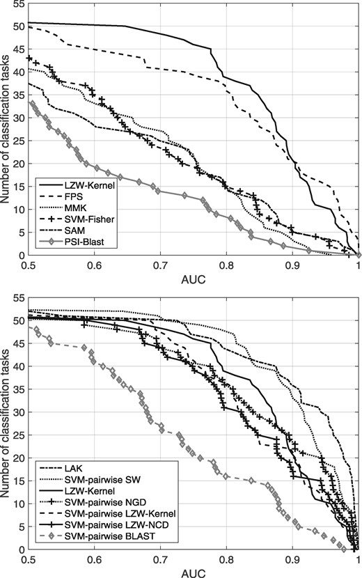
Comparison of LZW-Kernel to the baseline methods on the gold-standard dataset. Results are shown on two panels to avoid crowding. The plots show the total number of classification tasks for which a given method exceeds an AUC score threshold

4.4 Invariance to rearranged sequences

Protein evolution often includes domain rearrangements such as gain or loss of domains and circular shifts (Forslund and Sonnhammer, 2012; Moore et al., 2008). Therefore, the questions arise of how well the LZW-Kernel can detect such domain rearrangements. In order to study this, we used the C1S pre-cursor (UniProtKB/Swiss-Prot accession: P09871), a multi-domain of 688 residues consisting of a signal peptide (A), two CUB domains (B, B’), a EGF domain (C), two SUSHI domains (D, D’) and a trypsin-like catalytic domain (E) that is post-translationally cleaved from the pre-cursor. The domain architecture of the native protein can be written as ABCB’DD’E and a hypothetical circular shift can be written as DD’EABCB’. The results in Table 4 show how a reshuffling of the domains affects the LZW-Kernel, LZW-CBD, MMK, NGD, LAK and SW relative to the C1S sequence itself and to a random shuffled version of C1S. MMK seems to be quite blind to these domain rearrangements, as it can be expected from any amino acid composition based measure. Results also suggest that LAK is the most sensitive to these domain rearrangements. It cannot distinguish between a totally random sequence and a reversed or circularly shifted domain order. The SW is moderately sensitive to reverse order of domains and to circular shift; however, it is totally blind to sequence duplications. We consider LZW-CBD moderately sensitive and LZW-Kernel more sensitive to domain rearrangements. We note that the LZW-Kernel and LAK could be considered somewhat sensitive to sequence duplication; however, this is mainly due to normalization. The unnormalized LZW-Kernel function yields the same score of 1178 for (i) self-similarity of C1S protein and (ii) for the similarity between C1S and its duplicated version; however, (iii) it yields a low score of 384 when C1S is compared to its randomly shuffled version. The unnormalized LAK also yields very similar scores for (i) self-similarity (652.53) and (ii) for C1S and its duplicated version (677.15), but (iii) it yields a poor score (482.87) when C1S is compared to its randomly shuffled version. The NGD is insensitive to domain circulation and to reversed domain order, but it seems to be more sensitive to sequence length due to its normalization. For instance, the domain duplication causes more changes in the score then comparing a sequence to its randomly shuffled version. Whether insensitivity to domain rearrangement is an advantage or disadvantage depends on the application. We hope this study will provide a guide to program designers.

Table 4.

The effects of domain rearrangements on various measures

	LZW-Kernel		LZW-CBD		MMK-(5, 1)		NGD		LAK		SW
	score	%b	score	%b	score	%b	score	%b	score	%b	score	%b
Itself (ABCB’DD’E)a	1	0	0.646	0	1	0	0	0	1	0	1895	0
Duplication of C (ABCCB’DD’E)	0.975	5	0.659	11	0.976	2	0.058	15	0.975	10	1804	5
Deletion of C (ABB’DD’E)	0.928	15	0.657	09	0.965	4	0.063	16	0.972	11	1673	12
Deletion of CB’ (ABCB’DD’E)	0.835	35	0.689	35	0.875	13	0.234	62	0.889	43	1305	31
Circular shift (D’EABCB’D)	0.720	60	0.676	24	0.994	1	0.001	0.3	0.739	100.3	966	50
Reverse order (ED’DB’CBA)	0.709	62	0.659	11	0.959	4	0.031	8	0.755	94	679	65
Duplication (2xABCB’DD’E)	0.676	70	0.743	79	0.999	0	0.500	132	0.734	102	1895	0
Random shuffled	0.534	100	0.769	100	0.026	100	0.380	100	0.740	100	19	100

a

UniProtKB/Swiss-Prot accession: P09871, A = Signal peptide (res. 1-15), B, B’=CUB domains (res. 16-130, 175-290, respectively), C = EGF domain (res. 131-172), D, D’=Sushi domains (res. 292-356, 357-423, respectively), E = Peptidase S1 (res. 438-688).

b

Score of C1S with itself = 0%, score of C1S with randomly shuffled C1S = 100%.

4.5 Sequence clustering on the Alfree

We tested LAK, MMK, and our LZW-Kernel method against 38 (mainly alignment-free but including SW) sequence comparison measures on the Alfree benchmark dataset (Zielezinski et al., 2017) that was constructed based on the ASTRAL v2.06 dataset (Fox et al., 2013) from 6569 protein sequences organized into 513 family groups, 282 superfamilies, 219 folds and 4 classes. The clustering ability of the methods was measured by ROC analysis. The best-performing method here was the NGD, which achieved 0.760 mean AUC over the four groups, while SW and LAK achieved 0.720 and 0.758 mean AUC, respectively. The kernel functions MMK and LZW-Kernel performed rather poorly here; they achieved 0.637 and 0.645 mean AUC, respectively. However, if we employ the normalization technique used by NGD, $\tilde{k}=-(\max (k(x,x),k(y,y))-\min (k(x,x),k(y,y)\left)\right)/\left(k\right(x,y)-\min (k(x,x),k(y,y)\left)\right),$ then MMK and LZW-kernel achieve 0.723 and 0.739 mean AUC, respectively. Thus, we think the normalization has a key role in this type of evaluation scenario. The LZW-Kernel would be among the four best and six fastest methods in the Alfree benchmark dataset. Further details about normalization and timing results can be found in Supplementary Section S2.

5 Conclusions

In this article, we introduced a new convolutional kernel function, called LZW-Kernel, for protein sequence classification and remote protein homology detection. Our kernel function utilizes the code blocks identified by the universal LZW text-compressors and directly constructs a kernel function out of them, resulting in better computational properties than NCD. Therefore, it can be considered a bridge between the realms of kernel functions and compression based methods. The LZW-Kernel is extremely fast. In our experimental tests, we showed that LZW-Kernel can be twice as fast as the MMK, three times faster than the BLAST and several magnitudes faster than the dynamic programming based LAK function and the SW method. We also showed that LZW-Kernel outperforms the amino acid composition (n-gram) based MMK and the other gold standard methods used for protein homology detection such as Fisher kernel, the hidden Markov model based SAM, and the protein family-based methods such as PSI-BLAST and the FPS methods. It is quite surprising that, at a fraction of the time, the LZW-Kernel closely approaches the performance of the exhaustive LAK and the SVM-pairwise methods when the SW method is used as an underlying scoring function during the feature vector construction. Moreover, LZW-Kernel significantly outperforms the SVM-pairwise method when it is combined with BLAST. This is in fact surprising, because these methods use a rich biological knowledge encoded in the substitution matrix and gap penalties, while LZW-Kernel does not use a substitution matrix and/or gap penalties.

Finally, we mention that because the LZW-compressor is related to the entropy of the input string, the LZW-Kernel is likely to have an information-theoretic interpretation. For example, the symmetrized Kullback–Leibler divergence is a good candidate to characterize our kernel. Numerical simulations with Markov models point in this direction and a precise mathematical relationship is the topic of one of our ongoing research projects.

Conflict of Interest: none declared.