


Abstract
Machine learning plays a substantial role in bioscience owing to the explosive growth in sequence data and the challenging application of computational methods. Peptide-recognition domains (PRDs) are critical as they promote coupled-binding with short peptide-motifs of functional importance through transient interactions. It is challenging to build a reliable predictor of peptide-binding residue in proteins with diverse types of PRDs from protein sequence alone. On the other hand, it is vital to cope up with the sequencing speed and to broaden the scope of study.
In this paper, we propose a machine-learning-based tool, named PBRpredict, to predict residues in peptide-binding domains from protein sequence alone. To develop a generic predictor, we train the models on peptide-binding residues of diverse types of domains. As inputs to the models, we use a high-dimensional feature set of chemical, structural and evolutionary information extracted from protein sequence. We carefully investigate six different state-of-the-art classification algorithms for this application. Finally, we use the stacked generalization approach to non-linearly combine a set of complementary base-level learners using a meta-level learner which outperformed the winner-takes-all approach. The proposed predictor is found competitive based on statistical evaluation.
PBRpredict-Suite software: http://cs.uno.edu/~tamjid/Software/PBRpredict/pbrpredict-suite.zip.
Supplementary data are available at Bioinformatics online.
1 Introduction
With the exponential growth of biological data and the enormous complexities involved in their modeling, data mining and machine learning became essential for the modern life science research. Development of computational tools that can extract patterns from sequence data for which the true labels can only be determined through experimental structures is crucial in proteomics. As of June 2017, the RefSeq database (release 82) (Pruitt et al., 2007) of the National Center for Biotechnology Information (NCBI) contains 725 times more protein sequences than that of structures available in RCSB Protein Data Bank (PDB) (Berman et al., 2000). Therefore, prediction of biologically relevant patterns from sequence only through appropriately mining and modeling the available data using machine learning algorithms, can produce Supplementary Material at a faster rate. With a view to the above consideration, in this article, we attempt to build a stacking approach based ensemble model (Wolpert, 1992) to predict peptide-binding residues from protein sequence.
Protein–protein interactions (PPIs) play a key role in the biological processes as well as pathogenic processes in a living cell. A major portion of PPIs involve recognition of short peptides by globular Peptide-Recognition Domain (PRD) that can induce binding with peptides and can form transient complexes (London et al., 2010; Malhis and Gsponer, 2015). Human proteome contains millions of peptide-motifs that are typically disordered in an unbound state and undergo disorder-to-order transition while bound to appropriate partners. Peptide–protein interactions are involved in a wide range of molecular activities (Scott and Pawson, 2009; Toogood, 2002). Moreover, 22% of human disease mutations occur in disordered regions of proteins with such motifs (Uyar et al., 2014). The peptide-binding tendency of proteins with different PRDs can be utilized to scan a proteome to identify the peptide-motifs that may bind a PRD. Therefore, fast identification of peptide-binding residues or regions in proteins containing PRDs that promote transient interactions is a pre-requisite for identifying peptide-motifs and is crucial for assembling peptide-mediated interactomes.
Computational and experimental techniques have been developed and used to identify peptide–protein interactions (Chen et al., 2015; Franceschini et al., 2012; Weatheritt et al., 2012). However, the problem under consideration of this study is to identify the residue patterns in the protein sequence that can recognize short peptides. Given a protein’s structure, tools have been developed to predict peptide-binding sites, e.g. Pepsite (Petsalaki et al., 2009), Peptimap (Lavi et al., 2013), PepBind (Das et al., 2013). However, a sequence-based approach has further implications as most of the structures are unavailable. Despite much progress, the sequence-based computational efforts have been taken to predict a few PRDs, i.e. MHC molecules (Hoof et al., 2009; Nielsen and Andreatta, 2016). We found one tool in the literature called SPRINT (Taherzadeh et al., 2016) that predicts peptide-binding sites on multiple PRDs, i.e. MHC, PDZ, SH2, and SH3 from sequence.
For this study, we collected a set of protein complexes containing sequences with a wide range of PRDs, like MHC I/II, PDZ, SH2, SH3, WW, 14-3-3, Chromo and Bromo, Polo-Box, Phospho-Tyrosine Binding (PTB), Tudor, enzyme inhibitor, antibody-antigen and others. Using a comprehensive set of sequence-based features, we model the peptide-binding residue patterns in a variety of PRDs using a sophisticated ensemble technique, stacked generalization. The proposed peptide-binding residue predictor is named PBRpredict. Furthermore, we develop two complementary versions of the initial model by tuning the classification thresholds, keeping the other parameters and overall framework the same, to improve the model’s capacity to recognize potential binding sites. The final three models are called PBRpredict-strict, PBRpredict-moderate and PBRpredict-flexible, which are combined in the PBRpredict-Suite. We carried out rigorous performance evaluations of the developed models using statistical metrics and case-studies and found the suite effective in predicting peptide-binding residues from protein sequence.
2 Experimental setup
In this section, we describe the data preparation steps, including data collection, definition and annotation of peptide-binding residues and regions in protein sequence, aggregation of features to encode protein residues to identify binding residues and the statistics used for performance evaluation.
2.1 Data preparation
For this study, we collected a set of globular protein receptors which were experimentally found to bind with short peptide chains (5–25 residues long) in a complex. We explored PDB to assemble a set of peptide-protein complex structures using the following criteria: (i) experimental method: x-ray crystallography; (ii) molecule type: protein (no DNA, RNA or hybrid); (iii) number of chains (both asymmetric unit and biological assembly): ≥2 and (iv) structures with at least one 5–25-residues long chain. The residues of receptor proteins that are involved in peptide-binding are then annotated as binding (‘b’), otherwise as non-binding (‘n’).
Our initial search with above criteria resulted in 6043 protein complexes which contain in total 25 557 chains. We filtered the dataset to remove complexes that have one or more subunit chains with unknown amino acid residues, ‘X’ or ‘Z’, because the necessary chemical features (Meiler et al., 2001) are not available for these residues. Moreover, a multimeric protein (homomeric and heteromeric) can contain multiple entries of identical chains. In such cases, we kept only one unique copy of a chain that maximizes the number of peptide-binding residues. In the feature generation steps, we used SPINE-X (Faraggi et al., 2012) to generate predicted values of the two backbone angles, phi and psi. We removed those chains for which SPINE-X failed to produce the required features. Finally, we clustered the remaining sequences at sequence identity below 40%. From each cluster, a representative sequence with maximum peptide-binding residues was chosen in the non-redundant dataset of 644 receptor protein chains, named as rcp644, freely available within the software package.
2.1.1 Peptide-recognition domains in the dataset
A wide range of PRDs were included in the rcp644 dataset of receptor chains that mediate peptide–protein interactions, for example, the major histocompatibility complex (MHC I and II) domain can recognize peptide fragments derived from the pathogen. The PDZ domain generally binds to C-terminal peptide-motifs. The Src Homology 2 (SH2) and PTB domains recognize phosphorylation of tyrosine (pTyr or pY). The PTB domain can bind to the N-P-x-Y motif as well. The Src Homology 3 (SH3) domain binds to Pro-rich motifs and peptide-motifs, such as R-x-x-K. The 14-3-3, WW, Polo-box, BRCA1 C Terminus (BRCT), forkhead-associated (FHA) domains recognize different type phosphorylation or post-translational modifications (PTMs) of threonine (pThr or pT) and serine (pSer or pS). The chromatin organization modifier (Chromo), Bromodomain and Tudor domain bind to methylated or acetylated peptides, such as Tudor domain can recognize PTMs on lysine (meLys or meK) and arginine (meArg or meR) by methylation. Chromo domain can also recognize meLys and Bromo domain recognize PTMs on lysine by acetylation (acLys or acK). The enzyme/inhibitor complexes with hydrolase, kinase, isomerase, phosphatase, protease and so on. Further, we included antibody-antigen, amyloid fibrils, membrane or transmembrane protein and nuclear receptor complexes in the dataset. The count of sequences with different domains and the distribution of positive (peptide-binding) and negative (non-binding) class type residues of those sequences are reported in Supplementary Table S1.
2.1.2 Training and test sets
The training set is composed of 475 protein chains, named rcp_tr475. It contains 400 relatively longer chains (25 residues) and 75 shorter chains (25 residues). The set consists of 89 512 residues of which 12.0% (10 709 residues) were peptide-binding and rests (78 803) were non-binding residues. The training set was further divided into 2-folds (243 and 232 chains), in which we included 50% of the sequences with each PRD. These 2-folds were utilized to prepare meta-level training set using independent prediction outputs by base-level models (details in Section 3.2).
The independent test set contains 169 chains, called as rcp_ts169. It has 146 long chains and 23 short chains. Moreover, it has a total of 26 977 residues including 5162 (14.1%) peptide-binding samples (positive) and 21 815 (85.9%) non-binding samples (negative). The count of sequences with different PRDs included in the training and test sets is reported in the Supplementary Table S1.
2.2 Data mining and annotation
A putative interaction between two amino acids is determined based on their atomic distances in the crystal structure. Specifically, we annotated an amino acid residue as peptide-binding residue if at least one of its heavy atoms stays within six angstrom distance from a heavy atom of a peptide residue (Jones and Cozzetto, 2015). To consider the heavy atoms only, we ignored the hydrogen atoms while determining interactions. Further, we did not account two adjacent amino acids on the either side of a target residue to skip the covalent bonded stable interaction and stored only the transient interaction which was relevant with the induced-binding in a peptide-protein complex (Malhis and Gsponer, 2015).
After annotating the residues as either peptide-binding (‘b’) or non-binding (‘n’), we applied a smoothing strategy to have regions of binding residues. We smoothed-out maximum three-residue long non-interacting regions that fall within two consecutive interacting regions or residues. Therefore, we surmise that the resulting regions are the ‘potential’ areas that contain the residues of interaction. We call such labeling as synthetic annotation, which was assigned on top of the actual annotation. With synthetic annotation, the proportion of peptide-binding/non-binding residues in rcp644 dataset changed from 12.5/87.5 to 17.1/82.9%. Figure 1 shows a sample synthetic annotation of a chain with PDZ domain (PDB ID: 4JOE).
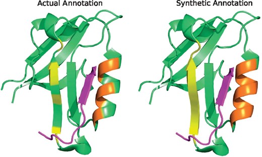
The actual (left) and synthetic (right) annotations of peptide-binding residues (highlighted) are shown on a protein’s (PDB ID: 4JOE) tertiary structure (green) bound to a peptide (pink). The binding residues of the two regions are marked in yellow and orange, respectively. Before smoothing, the binding residues were disjoint (left), whereas in synthetic annotation (right), the binding residues are contiguous. We viewed the 3D structure using PyMOL (Schrödinger, 2015) (Color version of this figure is available at Bioinformatics online.)
The rationale behind generating such synthetic annotation is: we have disjoint residues of interaction with non-interacting residues in between due to the geometrical orientation of the side chain atoms. Notwithstanding, it is tedious to capture these 3D structural details from 1D primary sequence alone and to subsequently guide a machine learning algorithm. To reduce the complexity, we localized the binding residues in a region so that the predictor-algorithm can be better informed about their characteristics from the sequential arrangement. In this way, we have less chance of missing a binding site as the contiguous residues can reinforce the residue-level as well as region-level prediction.
2.3 Feature set generation
We encoded the amino acid residues of the primary protein sequence using 60 features (f) of six groups as described below:
Residue profile (): the residue profile was created with the amino acid type and the terminal (t) residue indicator. A total of 20 different amino acids were encoded using 20 numbers. Further, we encoded five residues of N-terminal as and C-terminal as , respectively, whereas rest of the residues were labeled as 0.0. Thus, residue profile contributes two features per residue.
Chemical profile (f2–f8): seven physicochemical properties of amino acids were collected from Meiler et al. (2001).
Conservation profile (f9–f28, f37–f57): we executed three iterations of PSI-BLAST (Altschul et al., 1990) against NCBI’s non-redundant database to generate position specific scoring matrix (PSSM) of size sequence length, which gave us 20 features. These 1D scores given by PSSM was further extended to higher dimension by computing monogram (MG, 1 feature) and bigram (BG, 20 features) (Sharma et al., 2013). We used PSSMs, MG and BGs as conservation profile to predict peptide-binding residues.
Structure profile (f29 – f34): we used six sequence-based predicted structural properties; three secondary structure (SS) probabilities, specifically helix (H), beta (B) and coil (C), two backbone angles, phi () and psi (ψ), and one solvent accessible surface area (ASA) using tools called MetaSSpred (Islam et al., 2016), REGAd3p (Iqbal et al., 2015) and SPINE-X (Faraggi et al., 2012), respectively.
Flexibility profile (f35 – f36, f58): we created a flexibility profile with two backbone angle fluctuations, dphi () and dpsi (), and one disorder probability (drp) which were predicted using DAVAR (Zhang et al., 2010) and DisPredict (Iqbal and Hoque, 2015), respectively. These features are useful to capture the pattern of conformational changes that may result from coupled-binding between a short peptide and a globular receptor.
Energy profile (f59): the transient bonds between peptide and receptor involve formation and dissolution of atomic interactions that require change in free energy. To capture the state of free energy contribution of residues, we used Position Specific Estimated Energy (PSEE) which is computed from protein sequence (Iqbal and Hoque, 2016) using the pairwise contact energies from Miyazawa and Jernigan, 1985 and predicted ASA (Iqbal et al., 2015).
We further computed the importance of the individual features and analyzed the contribution of different feature categories in predicting peptide-binding residues, reported in the Supplementary Material, Section 4. The outcome suggested that the structural profile, flexibility profile and energy profile are the three most dominant feature categories; however, all the 60 features are useful. Thus, we used all 60 residue-wise features. Finally, we applied a sliding window of size 25 centering the target residue to include the properties of 12 residues on either side of the target, describing the local environment. Thus, we fed features per residue to train our predictor. The window size was selected through a separate set of experiments (see the Supplementary Material, Section 5).
2.4 Evaluation criteria
For the binary classification problem studied in this article, we consider the peptide-binding residues as the positive-class and the non-binding residues as the negative-class. Then, we computed the recall or sensitivity [true positive rate (TPR)], specificity [true negative rate (TNR)], fall-out or over-prediction rate [false positive rate (FPR)], miss rate TNR, balanced accuracy (ACC), precision (PPV), F1 score and Mathews correlation coefficient (MCC) to evaluate and compare the proposed predictor. Moreover, we plotted the he ROC curves and precision-recall curves, and computed the Area under ROC curve (AUC) to assess for probability assignment. The definition of the metrics are described in the Supplementary Material, Section 2.
3 Predictor framework
We applied stacked generalization (Wolpert, 1992) to develop the peptide-binding residue predictor (PBRpredict). Stacking is an ensemble technique to minimize the generalization error and has been successfully applied in several machine learning tasks (Nagi and Bhattacharyya, 2013). To the best of our knowledge, this study has first explored stacking for identifying the pattern of protein sequence that induces binding with peptides.
Stacking framework involves two-tier learning. The classifiers of the first tier and the second tier are called base-learner and meta-learner, respectively. Multiple base-learners are employed in the first tier. In the second tier, the outputs of the base-learners are combined using another meta-learner. Here, the underlying idea is: different base-learners can incorrectly learn different regions of the feature space, effectively due to the no-free-lunch theorem (Wolpert and Macready, 1997). A meta-learner, which is usually non-linear, is then applied to correct the improper training of the first tier. Thus, the meta-learner is trained to learn the error of the base-learners. Therefore, it is desirable to use classifiers as base-learners that can generate uncorrelated prediction outputs.
3.1 Base-level training and validation
We explored six different machine leaning algorithms as base-learners which are Support Vector Machine (SVM), Random Decision Forest (RDF), Extra Tree (ET) Classifier, Gradient Boosting Classifier (GBC), K Nearest Neighbors (KNN) and Bagging (BAG). The models were trained on the full rcp_tr475 dataset using features and were tested on the test dataset (rcp_ts169). Guided by the performance of these six algorithms (see Section 4.1), we finally employed SVM, GBC and KNN in the base-level of the stacking and used Logistic Regression (LogReg) as meta-learner to combine probability distributions generated at the base-level.
Let us assume, Ntrain and Ntest are the total number of residues of the training and test sets. Then the base-models, MODELSVM, MODELGBC and MODELKNN, were trained using the feature matrix of size where the per-residue feature vector was, . We tuned the parameters of SVM and developed the model using libSVM package (Chang and Lin, 2011), while the rest of classifier models were built and tuned using scikit-learn (Pedregosa et al., 2011). The algorithms and the involved parameters are described in the Supplementary Material, Section 3.
3.2 Meta-level training and validation
We used 63 per-residue features to train the meta-level learner; 3 probability outputs of MODELSVM (pSVM), MODELGBC (pGBC) and MODELKNN (pKNN), and the 60 features of the target residue. We combined the independent prediction outputs of the base-models into the training feature matrix for the meta-learner through blending, shown in Figure 2. We divided the train set of 475 chains into 2-folds of 243 and 232 chains so that . Here, and Nfold2 are the number of residues of 243 and 232 chains, respectively.
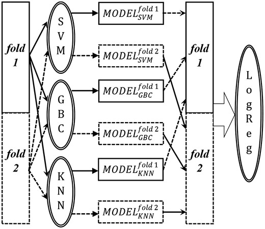
Blending of the outputs of SVM, GBC and KNN to generate independent prediction outputs on two different folds of the full training set. These outputs are then used as training features for the meta-level LogReg classifier. The objects and arrows associated with fold 1 and fold 2 are indicated by solid line and dashed line, respectively
At first, number of residues with M number of features were used to develop the three base models, which were used to predict Nfold2 number of residues. Conversely, Nfold2 number of residues with M number of features were used to develop another set of base models and the predicted probability values for number of residues were generated using these models. Thereafter, the independently predicted probabilities were combined to generate the data matrix of size to train the LogReg where the per-residue feature vector was, .
To test the meta-learner, we predicted the 169 chains of the test set by the MODELSVM, MODELGBC and MODELKNN which were trained using full training set and generated pSVM, pGBC and pKNN. With these three probabilities and the 60 features for Ntest number of residues, 169 chains were predicted by the meta-learner.
3.3 PBRpredict-Suite
PBRpredict-Suite is a collection of three PBRpredict models of similar framework, namely PBRpredict-strict, BRpredict-moderate, and PBRpredict-flexible, that were developed using same learning algorithms and feature set combinations in both levels of stacking. However, the predictors apply different threshold values to convert the probability outputs (or confidence score) into binary outputs. We named the predictors according to the imposed restriction level via thresholding in identifying the positive-class (peptide-binding residues).
Let us denote the set of thresholds used by SVM, GBC, KNN and LogReg as (tsvm, tgbc, tknn, tlogreg). With that, the definition of the three predictors within PBRpredict-Suite are given below.
PBRpredict-strict: the traditional value of 0.5 is used as thresholds by all the learners. Thus (tsvm, tgbc, tknn, tlogreg) = (0.5, 0.5, 0.5, 0.5).
PBRpredict-moderate: here, we apply a moderate set of values as thresholds, (tsvm, tgbc, tknn, tlogreg) = (0.3, 0.34, 0.35, 0.3).
PBRpredict-flexible: in this model, the classification thresholds for all the learners are further relaxed, (tsvm, tgbc, tknn, tlogreg) = (0.17, 0.21, 0.21, 0.2).
The framework of the PBRpredict-Suite is illustrated in Figure 3. The threshold values for the moderate and flexible models were statistically chosen to correct certain percentage of the false negative (FN) prediction outputs of the strict model (see Section 4.3). Moreover, the original probabilities given by the learners of moderate and flexible predictors are scaled to [0.5, 1.0] for positive-class and to [0.0, 0.5] for negative-class from the new range defined by the modified thresholds. Altogether, these three models performed promisingly in different cases (see Results). The models are implemented and integrated into a single PBRpredict-Suite software package, which outputs per-residue binary annotation and real-value probability. The software also outputs a summary file that reports the peptide-binding tendency per-chain averaged over the predicted peptide-binding residues and all residues.
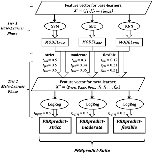
PBRpredict-Suite framework including PBRpredict-strict, PBRpredict-moderate and PBRpredict-flexible. The abbreviations used are explained in Section 3
4 Results
In this section, we report the results of parameter selection for the predictor models. Further, we discuss the performance of PBRpredict-Suite models and compare it with SPRINT (Taherzadeh et al., 2016).
4.1 Evaluation and analysis of the base learners
Here, we analyze the performances of the six classifiers, SVM, RDF, ET, GBC, KNN and BAG that we explored in the base-level of stacked generalization. The models were trained using rcp_tr475 dataset and were evaluated using independent test set, rcp_ts169. The predicted annotations were compared against the synthetic annotations of peptide-binding residues that were used to train the models.
Table 1 compares the binary prediction output of the learners and highlights that the optimized RBF-kernel SVM model gave outstanding performance in this application. The RBF-kernel SVM model gave the best recall (completeness of a classifier in predicting peptide-binding residues), miss-rate (rate of misclassifying a peptide-binding residue as non-binding), balanced accuracy (ACC) scores of values 0.547, 0.453 and 0.753. The closest competitor of SVM in terms of recall and ACC was the ET classifier.
Performance of the base-learners
| Metric | ET | RDF | SVM | GBC | KNN | BAG |
|---|---|---|---|---|---|---|
| Sensitivity/recall (TPR) | 0.418 | 0.365 | 0.547 | 0.373 | 0.348 | 0.398 |
| Specificity (TNR) | 0.977 | 0.982 | 0.959 | 0.977 | 0.965 | 0.981 |
| Fall-out rate (FPR) | 0.023 | 0.018 | 0.041 | 0.023 | 0.035 | 0.019 |
| Miss rate (FNR) | 0.582 | 0.635 | 0.453 | 0.627 | 0.652 | 0.602 |
| Accuracy (balanced) | 0.697 | 0.673 | 0.753 | 0.675 | 0.657 | 0.689 |
| Precision | 0.809 | 0.829 | 0.762 | 0.791 | 0.701 | 0.829 |
| F1_Score | 0.551 | 0.506 | 0.637 | 0.507 | 0.465 | 0.538 |
| MCC | 0.520 | 0.491 | 0.579 | 0.480 | 0.420 | 0.515 |
Note: Best score values are bold faced.
The RDF predicted the non-binding residues most accurately in terms of specificity (0.982) and BAG gave the best precision score of 0.829 (correctness of a classifier in predicting peptide-binding residues). However, SVM model outperformed the other predictors in terms of two critical measures used to assess a binary classifier, MCC (regarded as the most effective measure for binary classification on an imbalanced dataset) and F1 score (balances between correctness and completeness of a classifier) with values of 0.579 and 0.637, respectively. These scores are 11.35% and 15.62% better than those provided by the closest competitor, ET. On the other hand, GBC and KNN performed similarly, which were comparatively lower than the other predictors.
Figure 4 compares the ROC and precision-recall (PR) curves produced by the six base-learners. The ROC and PR curves can assess the performance of a classifier throughout its entire operating range by evaluating the probability distribution at different thresholds. The curves in Figure 4a illustrates that the ET and RDF gave the highest and the second-highest AUC values of 0.887 and 0.881, respectively. The SVM was a close competitor with AUC value of 0.879. The KNN provided the lowest AUC value of 0.789.
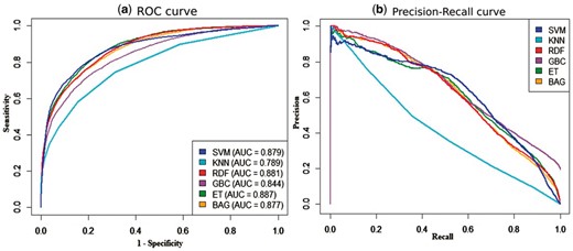
(a) ROC and (b) precision-recall curves given by six base-learners on peptide-binding residue prediction (rcp_ts169 dataset). The AUCs under the ROCs are given in the plot (a)
Figure 4a highlights the complementary competitiveness of SVM with RDF and ET classifier at different points. The sensitivity of SVM was lower than those of RDF and ET classifier at a range of high specificity (0.5–0.9), whereas at a range low specificity (0.0–0.45), SVM was better than RDF and ET. Another tree based ensemble learner, BAG showed a similar performance to those of RDF and ET. The PR curves in Figure 4b highlight that the precision of GBC, RDF and BAG were initially better than SVM and ET at a range low recall (0.0–0.4). However, SVM and ET gave better precision at higher recall (0.5–0.9). We also observed that the curves of KNN classifier were the least competitive.
We further performed a pair-wise correlation analysis of the residue-wise probabilities, given by these six learners on rcp_ts169 dataset, results reported in Table 2. We computed the Persons correlation coefficient () between the two sets of probabilities given by two classifiers. According to the working principle of stacking, it is desirable to use learners with complementary strengths in the base-level and therefore can provide uncorrelated outputs. In this way, the meta-level learner (LogReg) can learn about the improper training of the base-learners.
Pairwise correlation analysis of the probability distributions given by the base-learners on rcp_ts169
| Classifiers | ET | RDF | SVM | GBC | KNN | BAG |
|---|---|---|---|---|---|---|
| ET | — | 0.891 | 0.794 | 0.652 | 0.600 | 0.890 |
| RDF | — | — | 0.734 | 0.676 | 0.610 | 0.910 |
| SVM | — | — | — | 0.627 | 0.556 | 0.760 |
| GBC | — | — | — | — | 0.558 | 0.693 |
| KNN | — | — | — | — | — | 0.603 |
| Classifiers | ET | RDF | SVM | GBC | KNN | BAG |
|---|---|---|---|---|---|---|
| ET | — | 0.891 | 0.794 | 0.652 | 0.600 | 0.890 |
| RDF | — | — | 0.734 | 0.676 | 0.610 | 0.910 |
| SVM | — | — | — | 0.627 | 0.556 | 0.760 |
| GBC | — | — | — | — | 0.558 | 0.693 |
| KNN | — | — | — | — | — | 0.603 |
Note: Correlation values less than 0.7 are bold faced.
Table 2 shows that the tree-based ensemble learners, ET, RDF and BAG are highly correlated with each other, however, are less correlated with GBC, SVM and KNN. Therefore, a potential set of complementary learners is, ET, SVM, GBC and KNN. On the other hand, SVM is found less-correlated with GBC and KNN classifiers with correlation values of 0.627 and 0.556, respectively. Note that, from the results reported in Table 1, we found that SVM is the best representative classifier for this application and the GBC and KNN are less competitive. Therefore, another potential set is: SVM, GBC and KNN classifiers. We have further verified different sets of base-learners in the section below.
4.2 Evaluation of the stacked models
Here, we evaluated different set of base-learners and features at meta-level before finalizing PBRpredict model.
4.2.1 Combination of different base-learners
We evaluated four different combination of base-learners for stacked models (sM):
sM1 with ET, SVM, GBC, KNN, RDF and BAG (all six learners).
sM2 with ET, SVM, GBC and KNN. The RDF and BAG, which were highly correlated with ET (Table 2) are discarded.
sM3 with ET, SVM and GBC. The least performing KNN classifier while tested as a sole model is not considered in this set.
sM4 with SVM, GBC and KNN. Here, we combined the best performing base-learner, SVM with two relatively less competitive classifiers, GBC and KNN.
For all cases, the meta-level learner was LogReg, which was trained using rcp_tr475 dataset. Here, two different folds of the dataset were independently predicted by the base-learner models to generate probabilities while the models were trained on the other fold. Finally, the LogReg models were evaluated using independent test set, rcp_ts169.
The performance comparison among four stacked models, shown in Table 3, clarifies that our assumption about the effective set of base-learners was reasonable. The model using all six base-learners (sM1) was outperformed by the stacked models with reduced number of complementary base-learners. After removing BAG and RDF classifiers from the set (sM2), we got a slight improvement in MCC score. The sM3 with ET, SVM and GBC only provided the highest specificity/TNR (0.96) and precision (0.765) and the lowest fall-out rate (0.04). On the other hand, the stacking of SVM, GBC and KNN in sM4 gave the highest recall (TPR), ACC and F1 score of values 0.553, 0.756 and 0.640, respectively. We prioritized the balanced prediction capacity of a model in this classification task that can be measured by ACC and F1 score. Therefore, we utilized the base-learner set of sM4, SVM, GBC and KNN, to develop the PBRpredict-Suite predictors.
Comparison of stacked models with different set of base-learners on rcp_ts169 dataset
| sMs | TPR | TNR | FPR | FNR | ACC | PPV | F1 score | MCC | AUC |
|---|---|---|---|---|---|---|---|---|---|
| sM1 | 0.551 | 0.959 | 0.041 | 0.449 | 0.755 | 0.762 | 0.639 | 0.581 | 0.898 |
| sM2 | 0.551 | 0.959 | 0.041 | 0.041 | 0.755 | 0.762 | 0.640 | 0.582 | 0.897 |
| sM3 | 0.546 | 0.960 | 0.040 | 0.454 | 0.753 | 0.765 | 0.638 | 0.580 | 0.896 |
| sM4 | 0.553 | 0.959 | 0.041 | 0.447 | 0.756 | 0.760 | 0.640 | 0.581 | 0.886 |
Note: sM1 uses ET, SVM, GBC, KNN, RDF and BAG as base-learners.
sM2 uses ET, SVM, GBC and KNN as base-learners.
sM3 uses ET, SVM and GBC as base-learners.
sM4 uses SVM, GBC and KNN as base-learners.
Best values are marked in bold.
4.2.2 Combination of different features
During the selection of base-learners, results reported in Table 3, we used only the probability outputs generated from the base-learners as the features in the meta-level. Here, we further want to include additional features to boost up the capacity of meta-learner. We tested two different feature plans to train the meta-learner of sM4 stacked model that combines SVM, GBC and KNN.
Feature plan 1: contains the three probabilities generated by the base-learners only.
Feature plan 2: contains the 3 probabilities and the 60 features (Section 2.3) of the target residue.
The outputs of feature plan 1 and 2 were complementary, shown in Table 4. The meta-learner of plan 1 gave better specificity, which emphasizes the predictors’ capacity to identify non-binding residues. In contrast, the meta-model of plan 2 provided better recall that focuses the predictor’s ability to accurately identify the binding residues. Moreover, the model with feature plan 2 resulted in balanced prediction in terms of ACC, MCC and F1 score. Therefore, the PBRpredict-Suite models use SVM, GBC and KNN as the base-learners that were trained using features and LogReg as meta-learner that was trained using 63 features.
Comparison of stacked models with different set of features on rcp_ts169 dataset
| Feature set | Recall | Specificity | ACC | Precision | F1 score | MCC | AUC |
|---|---|---|---|---|---|---|---|
| Plan 1 | 0.553 | 0.959 | 0.756 | 0.760 | 0.640 | 0.581 | 0.886 |
| Plan 2 | 0.558 | 0.958 | 0.758 | 0.759 | 0.643 | 0.584 | 0.882 |
| Feature set | Recall | Specificity | ACC | Precision | F1 score | MCC | AUC |
|---|---|---|---|---|---|---|---|
| Plan 1 | 0.553 | 0.959 | 0.756 | 0.760 | 0.640 | 0.581 | 0.886 |
| Plan 2 | 0.558 | 0.958 | 0.758 | 0.759 | 0.643 | 0.584 | 0.882 |
Note: Best values are marked in bold.
4.3 Finalizing the PBRpredict-Suite models
In the proposed PBRpredict-Suite, we included three models to predict protein’s peptide-binding residues: PBRpredict-strict, PBRpredict-moderate and PBRpredict-flexible, which use different thresholds for classification. In this section, we discuss the development of these three different predictor models.
We named the stacked model sM4 with 63 features in the meta-level (Section 4.2) as PBRpredict-strict. This model provided a well-balanced performance when compared with the state-of-the-art predictor which is supported by both statistics (Section 4.4) and case-studies (Section 4.5). However, we call this model ‘strict’ in predicting the positive-class (peptide-binding residues) as it resulted in fine fall-out rate/FPR even at the cost of compromised recall score (TPR). Moreover, we observed that the PBRpredict-strict model provides conservative performance in identifying the binding residues in full-length sequence, relatively longer than the structure-specific shorter sequence, to avoid the false positive (FP) predictions or over-prediction (see Supplementary Fig. S4). Note that, we included only the structure-specific sequences from PDB in our training dataset, as we needed the experimental structures to extract the interaction information and annotate the protein sequence. However, we intend to design models that can identify peptide-binding sites in sequences with domains that are not known to the training set as well as within the full-length protein sequence with no experimentally solved structure. Therefore, we tuned our model further to improve the recall/TPR or positive-class prediction accuracy of our model.
We attempted to relax the classification threshold to recover the positive-class type (peptide-binding) residues that are falsely predicted as negative-class (non-binding). To understand the probabilistic behavior of the learners, we visualized the distributions of the probabilities generated by the classifiers for four different prediction types: true positives (TP), FP, true negative (TN) and FN using the threshold value 0.5 (see Supplementary Fig. S3). We noted that care must be taken in lowering the threshold from 0.5, which may convert certain TNs into FPs. We empirically observed such behavior of the classifiers in our experiments where we checked seven different threshold values: 0.45, 0.4, 0.35, 0.3, 0.25, 0.2 and 0.15 (results not shown). This experiment did not result in any certain value of the threshold as the recall continues to increase with the lower threshold value at a cost of very high over-prediction which is not desirable. Thus, we finally chose the thresholds according to certain statistics on the probabilities of FNs given by the classifiers as our aim is to correct FNs by assigning a different threshold to segregate the positive and negative-class.
We quantified the mean probabilities of FNs () along with the standard deviations () which are 0.172 ± 0.122 for SVM, 0.209 ± 0.130 for GBC, 0.208 ± 0.138 for KNN and 0.199 ± 0.105 for the LogReg. We checked the median values () as well which are 0.139 for SVM, 0.187 for GBC, 0.222 for KNN and 0.191 for the LogReg. Then, we considered the and values as different sets of thresholds.
We report the performances of SVM, GBC and KNN on rcp_ts169 dataset using these modified thresholds in the Supplementary Table S3. The results showed that for all the classifiers, the recall, miss-rate and accuracy (ACC) scores improved with lower threshold values. The models with the traditional threshold (0.5) produced the most balanced performance for SVM and KNN with the highest MCC scores. On the other hand, the models with thresholds equal to provided the best F1 scores for all the classifiers and the best MCC for GBC. Moreover, the fall-out or over-prediction rates with these threshold values were reasonable, specifically no >7.5%. On the other, the values were lower than the values for the SVM and GBC. Therefore, the use of values as thresholds resulted in outstanding recall scores, however at a cost of very high fall-out rate which was not desirable. In addition, the performances of KNN models with and as thresholds were similar. Therefore, we did not consider the value as the threshold in the meta-level.
In Table 5, we report the results of the stacked models with modified threshold values on the rcp_ts169 dataset. The stacked model for which the and the are used as thresholds for all the base-level and meta-level learners are named as PBRpredict-moderate and PBRpredict-flexible, respectively. The actual threshold values are reported in the footnote of Table 5.
Comparison of PBRpredict-Suite models on rcp_ts169 dataset
| Metric | PBRpredict- strict | PBRpredict- moderate | PBRpredict- flexible |
|---|---|---|---|
| Recall/TPR | 0.558 | 0.666 | 0.774 |
| Specificity/TNR | 0.958 | 0.915 | 0.841 |
| Fall-out rate/FPR | 0.042 | 0.085 | 0.159 |
| Miss rate/FNR | 0.442 | 0.334 | 0.226 |
| Accuracy/ACC | 0.758 | 0.790 | 0.808 |
| Precision | 0.759 | 0.649 | 0.536 |
| F1 score | 0.643 | 0.657 | 0.633 |
| MCC | 0.584 | 0.575 | 0.541 |
| AUC | 0.882 | 0.884 | 0.886 |
Note: Best values are bold faced.
PBRpredict-strict thresholds: SVM(0.5), GBC(0.5), KNN(0.5), LogReg(0.5).
PBRpredict-moderate thresholds: SVM(0.3), GBC(0.34), KNN(0.35), LogReg(0.3).
PBRpredict-flexible thresholds: SVM(0.17), GBC(0.21), KNN(0.21), LogReg(0.2).
The output shows that the PBRpredict-strict with the threshold value of 0.5 resulted in the lowest fall-out rate with the highest MCC score (a balanced measure to assess a binary classifier), however, the recall score was lower as well as the miss rate was higher than those of other models in the suite. In PBRpredict-moderate, the thresholds were relaxed and set to a relatively lower values, defined by the . Subsequently, the TPR was increased by 19.4% at a cost of 4.54% decrease in the TNR. In addition, the F1 score and ACC were also improved by 2.19 and 4.27% for the PBRpredict-moderate than those of PBRpredict-strict model. In the PBRpredict-flexible model, the thresholds were even further lowered and set to . Therefore, all the FN predictions (miss rate) of PBRpredict-strict with probability values greater than or equal to the were corrected by the PBRpredict-flexible at a cost of high fall-out rate of around 16%.
4.4 Performance comparisons
In this section, we compare the performance of PBRpredict-Suite models with SPRINT (Taherzadeh et al., 2016). SPRINT is a sequence-based predictor of protein-peptide binding residues that uses an SVM with optimized parameter set. Moreover, the dataset, model parameter set and feature set for SPRINT are different than those of PBRpredict. We ran SPRINT through its webserver on our test dataset, rcp_ts169. However, SPRINT server could generate the predictions on 146 sequences out of 169, and failed for the rest. Thus, we compared the performance of the proposed models with that of SPRINT (Taherzadeh et al., 2016) on the 146 sequences only.
The comparison while evaluated against the synthetic annotation (with smoothing) is reported in Table 6. We observed that SPRINT could result in higher recall value than that of PBRpredict-strict model. Note that, we named this model ‘strict’ as it does not compromise the rate of FP (fall-out rate) even at a cost of lower recall score. The recall score of PBRpredict-strict was found 10.69% lower than that of SPRINT. On the other hand, the fall-out rate of SPRINT, which defines the rate of miss-classification of non-binding residues as peptide-binding residues or tendency of over-prediction, was 86.52% higher than that of PBRpredict-strict. Moreover, the PBRpredict-strict gave more precise and balanced performance with 15.42, 138.34, 132.50 and 51.99% higher balanced accuracy (ACC), precision, F1 score and MCC, respectively than those given by SPRINT. Further, the PBRpredict-moderate and flexible overcomes the shortcomings of the strict model. The PBRpredict-moderate and flexible provided 7.3 and 25.3% higher recall scores than that of SPRINT, respectively, while keeping the fall-out rate 72.3 and 48.3% lower than that of SPRINT. Thus, the three models in together made the PBRpredict-Suite comprehensive in identifying peptide-binding residues.
Comparison of SPRINT and PBRpredict-Suite models, evaluated against synthetic annotation
| Performance | PBRpredict | PBRpredict | PBRpredict | SPRINT |
|---|---|---|---|---|
| Metric | Strict | Moderate | Flexible | — |
| Recall/TPR | 0.547 | 0.658 | 0.768 | 0.613 |
| Specificity/TNR | 0.958 | 0.915 | 0.841 | 0.692 |
| Fall-out rate/FPR | 0.042 | 0.085 | 0.159 | 0.308 |
| Miss rate/FNR | 0.453 | 0.342 | 0.232 | 0.387 |
| Accuracy/ACC | 0.753 | 0.786 | 0.804 | 0.652 |
| Precision | 0.754 | 0.642 | 0.529 | 0.316 |
| MCC | 0.576 | 0.567 | 0.534 | 0.248 |
| F1 score | 0.634 | 0.650 | 0.626 | 0.417 |
Note: Best values are bold faced.
In Table 7, we report the performance comparison while the predictions were evaluated against actual annotation (without smoothing). A similar result was obtained where SPRINT gave competitive recall and miss-rate with PBRpredict-strict and moderate, however at a cost of higher fall-out rate, specifically 77 and 62.2% higher than that of PBRpredict-strict and moderate. Notwithstanding, PBRpredict-flexible resulted in 12.1% higher recall score than that of SPRINT even with 38.12% lower fall-out rate. In addition, PBRpredict-Suite models gave a better balanced scores in case of assessing against actual annotation as well. Specifically, the ACC, precision, MCC and F1 score given by PBRpredict-strict were 6.79, 109.82, 74.72 and 43.99% higher than those of SPRINT, respectively. These differences in performance are even higher when SPRINT was compared with PBRpredict-moderate as this model gave the best MCC and F1 score. The surprisingly superior performance given by SPRINT only in case of recall when compared to PBRpredict-strict, despite falling far behind it in terms of balanced measures such as MCC and F1 score provides us a clue that SPRINT suffers from over-prediction problem.
Comparison of SPRINT and PBRpredict-Suite models, evaluated against actual annotation
| Performance | PBRpredict | PBRpredict | PBRpredict | SPRINT |
|---|---|---|---|---|
| Metrics | Strict | Moderate | Flexible | — |
| Recall/TPR | 0.544 | 0.662 | 0.776 | 0.692 |
| Specificity/TNR | 0.928 | 0.882 | 0.806 | 0.686 |
| Fall-out rate/FPR | 0.072 | 0.118 | 0.194 | 0.314 |
| Miss rate/FNR | 0.456 | 0.338 | 0.224 | 0.308 |
| Accuracy/ACC | 0.736 | 0.772 | 0.791 | 0.689 |
| Precision | 0.548 | 0.472 | 0.390 | 0.261 |
| MCC | 0.474 | 0.475 | 0.450 | 0.271 |
| F1 score | 0.546 | 0.552 | 0.519 | 0.379 |
Note: Best values are bold faced.
Figure 5 presents the ROC curves generated by SPRINT and PBRpredict-Suite models while the predictions are evaluated against both synthetic and actual annotations. The curves show the TPR (sensitivity)/FPR (one specificity) output pairs at different classification thresholds. The ROC curves given by different models of the PBRpredict-Suite nearly overlapped with each other. The curves highlight the strength of PBRpredict models in achieving a high TPR of 80% (rate of correct prediction of peptide-binding residues) at a very low rate (20%) of FPR. On the other hand, SPRINT gave TPR 80% at a cost of high FPR 60% only. This performance gap persists when the predictions are compared against the actual annotation as well. Therefore, the synthetic annotation of the non-binding residues (negative-class) as peptide-binding (positive-class) in between disjoint peptide-binding regions did not contribute to over-prediction, rather better guided a machine learning technique to identify the binding residues from collective information of the residues at close vicinity. Moreover, the AUC scores given by PBRpredict-Suite models were at least 24.7 and 13% higher than those of SPRINT while evaluated against synthetic and actual annotation, respectively.
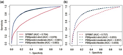
Comparison of ROC curves and AUC values given by SPRINT and PBRpredict-Suite models on 146 chains when evaluated against (a) synthetic and (b) actual annotation, indicated using solid and dotted lines, respectively. The AUC values under the ROCs are reported in the legend
4.5 Case-studies
4.5.1 Structure-specific sequences from rcp_ts169 dataset with known domains
Here, we performed case-studies with four different proteins with different PRDs. The structure-specific chains of these proteins were picked from rcp_ts169 test set that share less than 40% similarity with any chain of the training set. However, chains with similar domain type were present in the training set. We applied the PBRpredict-strict that uses the traditional threshold and SPRINT to predict the peptide-binding residue in each protein, and mapped the prediction outputs on the structure using PyMOL (Schrödinger, 2015). For a fair analysis and comparison on the structure-specific sequences, we applied the strictest model of the suite.
MHC-I Domain (PDB ID: 1LD9): here, we picked the 3D structure of an H-2Ld protein (green), shown in Figure 6, while interacting with a peptide (cyan). Prediction of PBRpredict-strict (Fig. 6b) for this case was perfect with recall and MCC of 1.0 and 0.99, respectively. On the other hand, the visual illustration of SPRINT prediction in Figure 6c shows the over-predicted binding residues (pink) throughout the full chain with a MCC of −0.123 and recall of 0.59.
SH2 Domain (PDB ID: 2CIA): Figure 7 shows the structure of human Nck2 protein with SH2 domain (green) in complex with a phosphotyrosine peptide (cyan). PBRpredict-strict (Fig. 7b) was statistically better than SPRINT (Fig. 7c) in this case with recall and MCC scores of 0.75 and 0.77, whereas these scores for SPRINT were 0.63 and 0.55, respectively.
Polo-Box Domain (PDB ID: 4LKL): Figure 8 shows crystal structure of the polo-like kinase with polo-box domain (green) in bound with five-residue long peptide (cyan). PBRpredict correctly predicted 89% of the peptide-binding residues (recall) and gave an MCC score of 0.76. To compare, SPRINT gave reasonable recall of 0.74, however, resulted in low MCC (0.23) due to over-prediction (Fig. 8c).
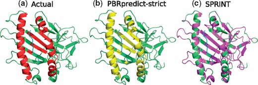
(a) Peptide-binding residues (red) of the MHC domain (green), bound to a peptide (cyan) in PDB 1LD9. The prediction outputs of PBRpredict-strict (yellow) and SPRINT (magenta) are shown in (b) and (c), respectively (Color version of this figure is available at Bioinformatics online.)
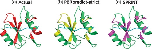
(a) Peptide-binding residues (red) of the SH2 domain (green), bound to a peptide (cyan) in PDB 2CIA. The prediction outputs of PBRpredict-strict (yellow) and SPRINT (magenta) are shown in (b) and (c), respectively (Color version of this figure is available at Bioinformatics online.)
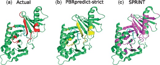
(a) Peptide-binding residues (red) of the Polo-Box domain (green), bound to a peptide (cyan) in PDB 4LKL. The prediction outputs of PBRpredict-strict (yellow) and SPRINT (magenta) are shown in (b) and (c), respectively (Color version of this figure is available at Bioinformatics online.)
4.5.2 Structure-specific sequences with unknown domains
In this section, we studied the performance of different PBRpredict-suite models in identifying peptide-binding residues of domains that are not known to the training set. We picked three domains for which no homologous are present in the training set: The malignant brain tumor (MBT) domain, VHS (VPS-27, Hrs and STAM) domain and CW domain. We collected the structures with these domains from PDB following similar steps described in Section 2.1. We respectively found 8, 9 and 10 structures of complexes in which chains with MBT, VHS and CW domains were bound to peptides. After filtering out the chains with a similar domain that shared >40% sequence similarity, we had 6, 4 and 7 sequences with MBT, VHS and CW domains, respectively. Then, we extracted the interaction information from the structures based on the atomic distance (Section 2.2) and annotated the structure-specific protein sequences. We performed these case-studies to understand the proposed model’s capacity to go beyond the PRDs that are known to the training set.
MBT Domain: The MBT domain recognizes the PTMs, i.e., methylation on lysine, on histone tails. The MBT domains are involved in transcriptional repression and have critical roles in diseases (Bonasio et al., 2010). Table 8a shows that the PBRpredict-strict model identified only 19.7% of the peptide-binding residues (TPR) of this domain, however, resulted in very low FPR. The moderate predictor could correct some of the incorrectly predicted binding residues, therefore the recall and accuracy scores improved with a reasonable FPR value of 0.081. On the other hand, the model with the most flexible threshold values resulted in the highest recall, ACC and F1 scores.
Table 8.Performance of PBRpredict-Suite models on unknown PRDs
Model TPR TNR FPR FNR ACC F1 score (a) MBT domain PBRpredict-strict 0.197 0.991 0.009 0.803 0.594 0.199 PBRpredict-moderate 0.351 0.919 0.081 0.649 0.635 0.319 PBRpredict-flexible 0.511 0.802 0.198 0.489 0.656 0.327 (b) VHS domain PBRpredict-strict 0.553 0.959 0.756 0.760 0.640 0.581 PBRpredict-moderate 0.558 0.958 0.758 0.759 0.643 0.584 PBRpredict-flexible 0.558 0.958 0.758 0.759 0.643 0.584 (c) CW domain PBRpredict-strict 0.553 0.959 0.756 0.760 0.640 0.581 PBRpredict-moderate 0.558 0.958 0.758 0.759 0.643 0.584 PBRpredict-flexible 0.558 0.958 0.758 0.759 0.643 0.584 Model TPR TNR FPR FNR ACC F1 score (a) MBT domain PBRpredict-strict 0.197 0.991 0.009 0.803 0.594 0.199 PBRpredict-moderate 0.351 0.919 0.081 0.649 0.635 0.319 PBRpredict-flexible 0.511 0.802 0.198 0.489 0.656 0.327 (b) VHS domain PBRpredict-strict 0.553 0.959 0.756 0.760 0.640 0.581 PBRpredict-moderate 0.558 0.958 0.758 0.759 0.643 0.584 PBRpredict-flexible 0.558 0.958 0.758 0.759 0.643 0.584 (c) CW domain PBRpredict-strict 0.553 0.959 0.756 0.760 0.640 0.581 PBRpredict-moderate 0.558 0.958 0.758 0.759 0.643 0.584 PBRpredict-flexible 0.558 0.958 0.758 0.759 0.643 0.584 Note: Best values are marked in bold.
VHS Domain: the VHS domains are mostly found in the N-terminal of many proteins and have crucial roles in membrane targeting (Lohi et al., 2002). VHS domain recognizes short peptide-motifs, i.e. D/ExxLL. The results, reported in Table 8b, show that the PBRpredict-flexible model recognized the highest number of peptide-binding residues of four VHS domain proteins with the highest recall (0.583), accuracy (0.576) and F1 score (0.354) values. On the other hand, the strict model gave the lowest recall score, however, almost perfectly predicted the non-binding residues with only two FPs (FPR: 0.004). The accuracy of the moderate model was in between the strict and flexible models.
CW Domain: the CW domain recognizes the lysine methylation on the N-terminal histone tails which have a key role in the tissue-specific gene expressions and chromatin regulations (Hoppmann et al., 2011). Table 8c shows the performances of the three PBRpredict-Suite models in recognizing the residue patterns of this domain averaged over seven chains. We observed a similar output where the strict and the flexible models recognized the lowest and the highest percentage of the binding residues, respectively. On the other hand, the PBRpredict-moderate model resulted in a modest recall value.
The results of the above case-studies on the domains that were unseen by the PBRpredict-Suite models during training advocate the strength of the proposed models in locating potential peptide-binding sites within sequences for which the cognate domains are not known to the models. Therefore, the predictors, especially the moderate and the flexible models, can be useful in determining possible peptide-binding sites from protein sequence when no putative interaction information is known. In the Supplementary Material (Section 7), we have further studied the performance of PBRpredict-Suite models on 53 protein chains that are independent of the training set.
4.5.3 Full-length sequences with unknown domains
In this section, we study the full-length protein sequences with PBRpredict-Suite models. Here, we want to evaluate the ability of the proposed models in identifying potential peptide-binding residues in proteins for which no experimental or template structure is available. For this study, we chose the Gid4 protein. Recently, Chen et al., 2017 discovered that the Gid4 subunit of the ubiquitin ligase GID in the yeast Saccharomyces cerevisiae targets the gluconeogenic enzymes, and recognizes the N-terminal proline (P) residue and the short five-residue-long adjacent sequence motifs. The authors Chen et al., 2017 identified such interactions through in vitro experiments with two-hybrid assays.
We computationally predicted the potential residues in the Gid4 protein that may mediate such interactions with gluconeogenic enzymes to degrade them and down-regulate the gluconeogenesis. We collected three Swiss-Prot reviewed proteins from UniProt, GID4_YEAST (ID: P38263), GID4_HUMAN (ID: Q8IVV7) and GID4_MOUSE (ID: Q9CPY6), and ran the PBRpredict-Suite models on these sequences to identify possible peptide-binding residues. As PBRpredict-strict model produce conservative output on full-length proteins (Supplementary Fig. S4), here we show the predicted peptide-binding residues given by PBRpredict-moderate and flexible only. We report the results on GID4_YEAST below and on GID4_HUMAN and GID4_MOUSE in the Supplementary Figures S8 and S9.
GID4_YEAST (UniProtKB – P38263): Figure 9a and b shows the possible binding residues in blue identified by the PBRpredict-moderate and PBRpredict-flexible model in GID4_YEAST. The moderate and flexible model found 34 and 71 binding-residue respectively with a similar average confidence of 0.58 (mean probability values generated for the binding residues).
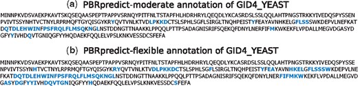
PBRpredict-moderate and PBRpredict-flexible annotation of peptide-binding residues in GID4_YEAST protein, shown in (a) and (b), respectively. The predicted binding residues are marked in blue (Color version of this figure is available at Bioinformatics online.)
The above case-studies show that the PBRpredict-Suite can be a useful tool in revealing the amino acid compositions that mediates crucial interactions with peptide-motifs from sequence alone when no structure is available. Such residue patterns can be further utilized for their cognate peptide identification. The above outcomes can further guide the experimental determination of the complex structure of these proteins by truncating the portion of the chain with potential peptide-binding sites.
5 Conclusions
In this paper, we presented the development and benchmarking of a suite of machine learning based PBRpredicts using protein sequence information alone. With the aim to model the residue patterns of a variety of PRDs, we collected and mined protein structure data to extract the true annotation. Three compatible learning algorithms, SVM, gradient boosting and KNN classifier, were trained using a set of intriguing features and the resulting models were further combined using logistics regression. Such model stacking technique better generalized the sequence pattern of diversified types of PRDs. The results and case-studies demonstrated that different PBRpredict-Suite models can generate well-balanced and biologically relevant predictions. Importantly, our evaluations showed that the proposed tool is capable of recognizing residue-patterns of unknown domains in different length sequences. Thus, it is worth utilizing the tool further in proteome-wide discoveries of new PRDs that can be verified experimentally.
Funding
This work was supported by the Board of Regents Support Fund, LEQSF (2016–2019)-RD-B-07.
Conflict of Interest: none declared.
References

