JRmGRN: joint reconstruction of multiple gene regulatory networks with common hub genes using data from multiple tissues or conditions

Abstract

Motivation

Joint reconstruction of multiple gene regulatory networks (GRNs) using gene expression data from multiple tissues/conditions is very important for understanding common and tissue/condition-specific regulation. However, there are currently no computational models and methods available for directly constructing such multiple GRNs that not only share some common hub genes but also possess tissue/condition-specific regulatory edges.

Results

In this paper, we proposed a new graphic Gaussian model for joint reconstruction of multiple gene regulatory networks (JRmGRN), which highlighted hub genes, using gene expression data from several tissues/conditions. Under the framework of Gaussian graphical model, JRmGRN method constructs the GRNs through maximizing a penalized log likelihood function. We formulated it as a convex optimization problem, and then solved it with an alternating direction method of multipliers (ADMM) algorithm. The performance of JRmGRN was first evaluated with synthetic data and the results showed that JRmGRN outperformed several other methods for reconstruction of GRNs. We also applied our method to real Arabidopsis thaliana RNA-seq data from two light regime conditions in comparison with other methods, and both common hub genes and some conditions-specific hub genes were identified with higher accuracy and precision.

Availability and implementation

JRmGRN is available as a R program from: https://github.com/wenpingd.

Supplementary information

Supplementary data are available at Bioinformatics online.

1 Introduction

Though all cells in a multicellular organism carry out some common processes that are essential for survival, different tissues can exhibit some unique patterns in gene expression that helps define their phenotypes. In addition, some organisms like plants may experience various environmental conditions in particular stresses. These common and tissue/condition-specific processes are ultimately controlled by GRNs that contain both common and tissue/condition-specific hubs. These hubs play critical roles for organisms to complete their life cycle. For example, abiotic and biotic stresses-responsive genes in rice have 70% in common and these genes showed conserved expression status, and the majority of the rest were down-regulated in abiotic stresses and up-regulated in biotic stresses (Shaik and Ramakrishna, 2014), indicating the presence of common hubs and network between two conditions. The local GRNs for different environmental conditions have been built in Arabidopsis (Barah et al., 2016; Hickman et al., 2013). Tissue-specific genes for 38 tissues have been identified in humans and the GRNs for each of these 38 tissues in humans have been built (Sonawane et al., 2017) and analyzed.

Comparison of global GRNs (Boyle et al., 2014) has revealed that the GNRs are largely conserved and share remarkable commonalities though they can change in response to environmental stimuli or at different tissue types. The high similarity in GRNs is primarily caused by the relatively smaller number of tissue/condition-specific nodes, for example, 23.4% genes were indicated to be tissue-specific (with complicity equal to one) after studying multiple tissues of humans (Sonawane et al., 2017). However, some local GRNs may be subject to some local topology changes (Faisal and Milenkovic 2014; Martin et al., 2016), making some regulatory interactions exist in all tissues or conditions while some others exist only in specific tissue or specific treatment.

Therefore, identification of both common and tissue- or condition-specific gene regulation provides key insights into complex biological systems (Tian, et al., 2016). In the past two decades, advances in microarray and RNA-seq technology have led to the generation of enormous wealth of gene expression data across various cell/tissue types and conditions. Although these datasets provide valuable opportunity to more robustly reconstruct condition-specific GRNs, there are very limited methods for modeling the complicated GRNs with high accuracy. Advanced and highly efficient methods are still in great demand.

Gaussian graphical models (GGMs) are widely used to reconstruct gene networks using gene expression data (Kumari et al., 2016). The models assume that gene expression data on $\mathrm{p}\mathrm{ }$genes from each sample follows a multivariate normal distribution with mean $\mathrm{\mu }$ and covariance matrix $\mathrm{\Sigma }$⁠, where $\mathrm{\mu }$ is a vector with $\mathrm{p}$ elements and $\mathrm{\Sigma }\mathrm{ }$is a $\mathrm{p}\hspace{1em}\times \hspace{1em}\mathrm{p}$ positive definite matrix. The conditional independence of two genes given other genes corresponds to a zero entry in the inverse covariance matrix ${\mathrm{\Sigma }}^{-1}$ (also called the precision or concentration matrix) (Lauritzen, 1996). Usually, we set $\mathrm{\Theta }={\mathrm{\Sigma }}^{-1}$⁠, called precision matrix or concentration matrix. Gaussian graphical models have the advantage of reconstructing direct dependencies between genes that represent edges in the reconstructed network: an edge corresponds a non-zero entry in ${\mathrm{\Sigma }}^{-1}$⁠. A natural way to estimate ${\mathrm{\Sigma }}^{-1}$ is by maximizing the log-likelihood of the data, which result in an estimation of precision matrix $\widehat{\mathrm{\Theta }}={\mathrm{S}}^{-1}$ where $\mathrm{S}$ is the sample covariance matrix.

However, directly applying GGM to reconstruct GRN is not applicable due to two problems. First, since the number of samples (⁠$\mathrm{n}$⁠) is generally much less than the number of genes (⁠$\mathrm{p}$⁠) from gene expression data, the sample covariance matrix $S$ becomes singular and thus it is impossible to computing the inverse. Second, even if the sample covariance matrix is not singular, the elements in the estimated precision matrix $\widehat{\mathrm{\Theta }}$ are in general not exactly equal to zero. For these reasons, Yuan and Lin (Lin et al., 2007) proposed to maximize a $\mathrm{L}1$ regularized log-likelihood function. Similar to LASSO regression (Tibshirani, 1996), they put a penalization on the sum of absolute value of each element in precision matrix, which leads to a sparse and positive definite estimation of $\mathrm{\Theta }$⁠.$\mathrm{ }$GLASSO (Friedman et al., 2008) is a fast algorithm to solve this optimization problem.

When applying GGMs to reconstruct gene regulatory networks, the underlying assumption is that each observation is drawn from the same distribution. However, when the gene expression data come from different tissues or under different treatments, this assumption is inappropriate. In this case, if one insists on modeling the gene expression data by one GRN, the results would be dubious and we cannot obtain the differential network e are interested in. A straightforward method to obtain the differential network is to reconstruct the network of each condition separately and then find the difference between them. However, this procedure ignores the similarity shared between GRNs across different tissues/treatments, which is critically important to reconstruct the GRNs, especially when the sample size is small. To reconstruct these dependent GRNs, Guo et al. (2011) proposed a joint penalized model using a hierarchical penalty and derived the convergence rate and sparsity properties of the resulting estimators. Danaher et al. (2014) proposed a joint graphical lasso model (JGL) to estimate multiple GRNs simultaneously. They proposed a fused graphical lasso penalization and a group graphical lasso penalization in addition to the sparsity penalization. In fused graphical lasso, the corresponding elements in the precision matrices are encouraged to have the same values. In group graphical lasso, the precision matrices in different conditions are encouraged to have similar sparsity pattern.

The above-mentioned methods do not impose any structural information of gene networks. That is, each gene has approximately the same number of interactions within the network, and each pair of nodes has equal probability to be an edge and all edges are independent. However, recent evidence points to scale-free properties in biological networks (Han et al., 2004; van den Heuvel and Sporns, 2013), in which most genes interact with a few partners whereas a small proportion of genes, called hub genes, are densely-connected to many other genes (high connectivity). To incorporate hub genes in GRNs, Liu and Ihler (2011) replaced the $\mathrm{l}1$ regularization in GLASSO with a power law regularization and optimized the objective function by solving a sequence of iteratively reweighted $\mathrm{l}1$ regularization problems, where the regularization coefficients of nodes with high degree were reduced, which encouraged the appearance of hub genes. Tan et al. (2014) introduced a row-column overlap norm penalty to incorporate hub genes explicitly. In their model, called hub graphical lasso (HGLASSO), the precision matrix $\mathrm{\Theta }$ was decomposed into two parts, one is elementary matrix $\mathrm{Z}$⁠, the other is hub matrix $\mathrm{V}$⁠, where $\mathrm{Z}$ is a symmetric matrix that is encouraged to be sparse, $\mathrm{V}$ is a matrix whose columns are encouraged to be either entirely zero or almost entirely non-zero through the $\mathrm{l}1/\mathrm{l}\mathrm{q}$ norm penalization. The non-zero columns of $\mathrm{V}$ correspond to hub genes. A detailed description of existing GGM related methods (GLASSO, JGL and HGLASSO) are given in Supplementary File 1 (S1).

The aim of this research is to develop new and more accurate method for: (i) construction of GRNs containing the important common hubs that may play essential roles for survival and/or adaptation; (ii) construction of GRNs containing tissue/condition-specific regulatory relationships that help us to understand phenotypes/traits of interest. In this manuscript, we assumed that a network for a specific tissue/condition can be decomposed into an elementary network that is unique to the tissue/condition, and a common network centered on hub genes that is shared across multiple tissues/conditions. Based on this hypothesis, we proposed a new method to jointly reconstruct multiple GRNs for multiple tissues/conditions in just one effort. Our method, JRmGRN, is different from the aforementioned methods. The methods from Yuan and Lin (Lin et al., 2007), Danaher et al. (2014) cannot model hub genes. Although the methods from Liu and Ihler (2011) and Tan et al. (2014) can be used to model hub genes, their methods are dedicated to reconstruction of a gene network from each dataset independently. With the availability of enormous amount of gene expression data from multiple tissues/conditions in public repositories, it is important to use datasets from multiple tissues or conditions together to identify common hub genes across multiple tissues or conditions and some tissue- or condition-specific hub genes, which will advance our understanding on regulation of biological processes and pathways. Our method hypothesizes that there are common hub genes in different tissues or under different environmental conditions. Figure 1 illustrates two example networks obtained from two tissues or conditions. There are many common edges (dash green) between two networks and some tissue- or condition-specific edges belonging to only one of the two networks (e.g. solid red and solid blue).

Fig. 1.

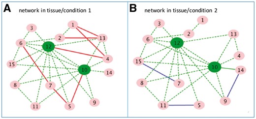
A toy example of two gene regulatory networks from two tissues or environmental conditions. Gene 10 and 12 are common hub genes in both networks. There are some edges (dash green) shared by the two networks and some edges (solid red or solid blue) belonging only to one network (Color version of this figure is available at Bioinformatics online.)

2 Materials and methods

2.1 Gaussian graphical model and regularization

Suppose that there are $\mathrm{K}$ datasets, ${\mathrm{Y}}^{\left(1\right)},\dots ,\mathrm{ }{\mathrm{Y}}^{\left(\mathrm{K}\right)}$⁠, where $\mathrm{K}\hspace{1em}\ge \hspace{1em}2$⁠, to represent gene express data from K tissues or conditions. ${\mathrm{Y}}^{\left(\mathrm{k}\right)}$ is a ${\mathrm{n}}_{\mathrm{k}}\times \mathrm{p}$ matrix where ${\mathrm{n}}_{\mathrm{k}}$ is the number of samples and $\mathrm{p}$ is the number of genes in the $\mathrm{k}$th dataset. Additionally we assume that the rows of ${\mathrm{Y}}^{\left(\mathrm{k}\right)}$ are independent and each row of ${\mathrm{Y}}^{\left(\mathrm{k}\right)}\sim \mathrm{N}({\mathrm{\mu }}_{\mathrm{k}},\mathrm{ }{\mathrm{\Sigma }}_{\mathrm{k}})(\mathrm{k}\hspace{1em}=\hspace{1em}1,\dots ,\mathrm{ }\mathrm{K})$⁠. Denote ${\mathrm{S}}^{\left(\mathrm{k}\right)}=\frac{1}{{\mathrm{n}}_{\mathrm{k}}}\left({\mathrm{Y}}^{\left(\mathrm{k}\right)}-{\mathrm{\mu }}_{\mathrm{k}}\right)\mathrm{\prime }({\mathrm{Y}}^{\left(\mathrm{k}\right)}-{\mathrm{\mu }}_{\mathrm{k}})$ as the sample covariance matrix of ${\mathrm{Y}}^{\left(\mathrm{k}\right)}$⁠. The precision matrix, ${\mathrm{\Theta }}^{\left(\mathrm{k}\right)}$ is the inverse matrix of the covariance matrix ${\mathrm{\Sigma }}_{\mathrm{k}}$⁠. For a gene regulatory network, the non-zero element ${\mathrm{\theta }}_{\mathrm{i}\mathrm{j}}^{\left(\mathrm{k}\right)}(\mathrm{i}\hspace{1em}\ne \hspace{1em}\mathrm{j})$ in ${\Theta }^{\left(\mathrm{k}\right)}$ indicate there is a conditional correlation between gene $\mathrm{i}$ and $\mathrm{j}$ for the $\mathrm{k}$th tissue/condition. Since the number of genes, $\mathrm{p}$⁠, is large and only a small portion of genes are associated, most of elements in ${\mathrm{\Theta }}^{\left(\mathrm{k}\right)}$ are expected to be zero. In addition, a few (hub) genes are expected to be associated with many other genes for different tissues or conditions, so the precision matrix ${\mathrm{\Theta }}^{\left(\mathrm{k}\right)}$ can be decomposed into two parts: one represents the elementary network for the $\mathrm{k}$th tissue/condition and the other part represents the network for hub genes. Based on such sparsity and decomposition of ${\mathrm{\Theta }}^{\left(\mathrm{k}\right)}$⁠, we propose the joint reconstruction of multiple gene regulatory networks with common hubs (JRmGRN) by solving the following penalized log-likelihood function,

$$\begin{array}{l}\left\{\begin{array}{l}\arg {\mathrm{m}\mathrm{i}\mathrm{n}}_{\left\{\begin{array}{l}{\mathrm{\Theta }}^{\left(\mathrm{k}\right)}\in {\mathcal{S}}^{+}, \\ k=1,.., K\end{array}|\}\right\}}\{\sum _{\mathrm{k}=1}^{\mathrm{K}}-{\mathrm{n}}_{\mathrm{k}}\left(\mathrm{l}\mathrm{o}\mathrm{g}\left(\mathrm{d}\mathrm{e}\mathrm{t}{(\mathrm{\Theta }}^{\left(\mathrm{k}\right)}\right))-\mathrm{t}\mathrm{r}\mathrm{a}\mathrm{c}\mathrm{e}\left({\mathrm{S}}^{\left(\mathrm{k}\right)}{\mathrm{\Theta }}^{\left(\mathrm{k}\right)}\right)\right)\\ +P\left(\right\{\Theta \left\}\right)\}\\ P\left(\{\mathrm{\Theta }\right\})={\mathrm{\lambda }}_1\sum _{\mathrm{k}=1}^{\mathrm{K}}{\left|\left|{\mathrm{Z}}^{\left(\mathrm{k}\right)}-\mathrm{d}\mathrm{i}\mathrm{a}\mathrm{g}\left({\mathrm{Z}}^{\left(\mathrm{k}\right)}\right)\right|\right|}_1\\ +{\mathrm{\lambda }}_2\sum _{\mathrm{k}<{\mathrm{k}}^{\mathrm{\prime }}}{\left|\left|{\mathrm{Z}}^{\left(\mathrm{k}\right)}-{\mathrm{Z}}^{\left({\mathrm{k}}^{\mathrm{\prime }}\right)}\right|\right|}_1+{\mathrm{\lambda }}_3{\left|\left|\mathrm{V}\right|\right|}_1+{\mathrm{\lambda }}_4{\left|\left|\mathrm{V}\right|\right|}_{1,2}\end{array}\right\}\end{array}\}$$

(2.1)

where ${\mathrm{Z}}^{\left(\mathrm{k}\right)}+\mathrm{V}+{\mathrm{V}}^{\mathrm{T}}={\mathrm{\theta }}^{\left(\mathrm{k}\right)}$ for $\mathrm{ }\mathrm{k}\hspace{1em}=\hspace{1em}1,\dots ,\mathrm{ }\mathrm{K}$ and ${\mathcal{S}}^{+}$ as the collection of symmetric positive semidefinite matrix. In the above penalized function. ${\left|\right|\mathrm{V}\left|\right|}_1=\sum _{\mathrm{i}\mathrm{j}}\left|{\mathrm{v}}_{\mathrm{i}\mathrm{j}}\right|$ denotes the sum of the absolute value of each element in $\mathrm{V}$⁠. $\mathrm{ }{\left|\right|\mathrm{V}\left|\right|}_{1,\mathrm{ }2}={\sum }_{\mathrm{j}\hspace{1em}=\hspace{1em}1}^{\mathrm{p}}{\left|\right|{\mathrm{V}}_{\mathrm{j}}\left|\right|}_2$ where ${\mathrm{V}}_{\mathrm{j}}$ is the ${\mathrm{j}}^{\mathrm{t}\mathrm{h}}$ column of matrix $\mathrm{V}$⁠. So ${\left|\right|\mathrm{V}\left|\right|}_{1,2}$ denotes the sum of the $l2$ norm of each column in $\mathrm{V}$⁠. In (2.1), the first part is the log-likelihood function of the data based on the precision matrix and the second part is the penalized function with $\mathrm{l}1$ norm to help us model the sparsity of ${\mathrm{\Theta }}^{\left(\mathrm{k}\right)}$⁠. We decompose the precision matrix ${\mathrm{\Theta }}^{\left(\mathrm{k}\right)}$ under the $\mathrm{k}$th tissue/condition into two parts: ${\mathrm{Z}}^{\left(\mathrm{k}\right)}$ and $\mathrm{V}$⁠. ${\mathrm{Z}}^{\left(\mathrm{k}\right)}$ can be seen as the elementary network under the $\mathrm{k}$th tissue/condition. $\mathrm{V}$ represents common hub genes across all tissues/conditions. We used four items in the penalized log-likelihood function $\mathrm{P}\left(\left\{\mathrm{\Theta }\right\}|\}\right)$ to ensure the reconstructed networks satisfied the desired properties. We summarized the purpose and the prior assumption of the four penalties in following:

1. ${\mathrm{\lambda }}_1{\sum }_{\mathrm{k}=1}^{\mathrm{K}}{\left|\left|{\mathrm{Z}}^{\left(\mathrm{k}\right)}-\mathrm{d}\mathrm{i}\mathrm{a}\mathrm{g}\left({\mathrm{Z}}^{\left(\mathrm{k}\right)}\right)\right|\right|}_1$⁠. The prior assumption is that elementary network under each condition is sparse, meaning that most of elements in ${\mathrm{Z}}^{\left(\mathrm{k}\right)}$ is zero. Therefore, we use $l1$ penalty to encourage the off diagonal elements of ${\mathrm{Z}}^{\left(\mathrm{k}\right)}$ to be zero.

2. ${\mathrm{\lambda }}_2\sum _{\mathrm{k}<{\mathrm{k}}^{\mathrm{\prime }}}{\Vert {\mathrm{Z}}^{\left(\mathrm{k}\right)}-{\mathrm{Z}}^{\left({\mathrm{k}}^{\mathrm{\prime }}\right)}\Vert }_1$⁠. The prior assumption is that each ${\mathrm{Z}}^{\left(\mathrm{k}\right)}$ contains some unique edges, representing the specific network for the kth ${\mathrm{k}}^{\mathrm{t}\mathrm{h}}$tissue/condition; but $\left\{{\mathrm{Z}}^{\left(\mathrm{k}\right)}\right\}$ have many common edges due to similarity among networks. Therefore, we use $l1$ penalty to encourage the elementary networks across different conditions to be the same.

3. ${\mathrm{\lambda }}_4{\left|\left|\mathrm{V}\right|\right|}_{1,2}$⁠. We assume matrix $\mathrm{V}$ contains zero columns and dense non-zero columns, where the non-zero columns represent the common hub genes across all tissues/conditions. Therefore, we use group lasso penalty to force some columns of $\mathrm{V}$ to be zero columns.

4. ${\mathrm{\lambda }}_3{\left|\left|\mathrm{V}\right|\right|}_1$⁠. For the non-zero columns of $\mathrm{V}$⁠, we also use $l1$ penalty to encourage some elements to be zero, so a hub gene will not connect to all other genes.

${\mathrm{\lambda }}_1,{\mathrm{\lambda }}_2,{\mathrm{\lambda }}_3\mathrm{ }\mathrm{ }\mathrm{a}\mathrm{n}\mathrm{d}\mathrm{ }{\mathrm{\lambda }}_4$⁠, are non-negative tuning parameters. Note that our model is different from methods that use Gaussian graphical model and regularization to reconstruct gene associate networks (Friedman et al., 2008; Lin et al., 2007). For example, GLASSO can only use data from single tissue or condition and cannot model hub genes (Friedman et al., 2008). JGL can use data from multiple tissues or conditions but cannot model hub genes (Danaher et al., 2014). HGLASSO incorporates hub genes in the reconstruction of gene networks but only handles data from a single tissue or condition (Tan et al., 2014). Although we may reconstruct gene networks for each tissue or condition using GLASSO/JGL/HGLASSO then use reconstructed networks to identify common hub genes, such approach is subjective and less efficient. In contrast, our proposed method is to reconstruct gene networks with hub genes by jointly using datasets from multiple tissues/conditions, thus is more efficient, powerful and accurate.

2.2 Algorithm to estimate parameters

For fixed values of tuning parameters ${\mathrm{\lambda }}_1,{\mathrm{\lambda }}_2,{\mathrm{\lambda }}_3\mathrm{ },{\mathrm{a}\mathrm{n}\mathrm{d}\mathrm{ }\mathrm{\lambda }}_4$⁠, the expression of (2.1) is a convex optimization problem, which can be solved by efficient algorithms available. The convexity of (2.1) can be proved by the following facts: the function of negative log determinant is a convex function, the norm functions are convex functions, and the nonnegative combination of convex functions is a convex function. We solved the problem (2.1) using the alternating directions method of multipliers (ADMM) algorithm, which allows us to decouple some of the terms in (2.1) that are difficult to optimize jointly. For more details on ADMM algorithm and its convergence properties, please consult the previous publication (Boyd et al., 2011).

We write the expression of (2.1) as a convex minimization problem with two blocks of variables and two separable functions as follows:

$$\begin{array}{l}\min \mathrm{\varphi }\left(\mathrm{X}\right)+\mathrm{\psi }\left(\stackrel{\sim }{\mathrm{X}}\right) s.t. X-\stackrel{\sim }{\mathrm{X}}=0 \end{array}$$

(2.2)

where $\mathrm{X}=\left({\mathrm{\Theta }}^{\left(\mathrm{k}\right)},\mathrm{ }{\mathrm{Z}}^{\left(\mathrm{k}\right)},\mathrm{ }\mathrm{V}\right),\mathrm{ }\stackrel{\sim }{\mathrm{X}}=\left({\stackrel{\sim }{\mathrm{\Theta }}}^{\left(\mathrm{k}\right)},\mathrm{ }{\stackrel{\sim }{\mathrm{Z}}}^{\left(\mathrm{k}\right)},\stackrel{\sim }{\mathrm{V}}\right)$⁠, and

$$\begin{array}{l}\varphi \left(\mathrm{X}\right)=f\left({\mathrm{\Theta }}^{\left(\mathrm{k}\right)}\right)+g\left({\mathrm{Z}}^{\left(\mathrm{k}\right)}\right)+h\left(\mathrm{V}\right)\end{array}$$

(2.3)

$$\begin{array}{l}\psi \left(\stackrel{\sim }{\mathrm{X}}\right)=\sum _{\mathrm{k}=1}^{\mathrm{K}}\mathrm{I}\left({\stackrel{\sim }{\mathrm{\Theta }}}^{\left(\mathrm{k}\right)}=\mathrm{ }{\stackrel{\sim }{\mathrm{Z}}}^{\left(\mathrm{k}\right)}+\stackrel{\sim }{\mathrm{V}}+{\stackrel{\sim }{\mathrm{V}}}^{\mathrm{\prime }}\right)\end{array}$$

(2.4)

where

$$\begin{array}{l}f\left({\mathrm{\Theta }}^{\left(\mathrm{k}\right)}\right)=\sum _{\mathrm{k}=1}^{\mathrm{K}}-{\mathrm{n}}_{\mathrm{k}}\left(\mathrm{l}\mathrm{o}\mathrm{g}\mathrm{d}\mathrm{e}\mathrm{t}{\mathrm{\Theta }}^{\left(\mathrm{k}\right)}-\mathrm{t}\mathrm{r}\mathrm{a}\mathrm{c}\mathrm{e}\left({\mathrm{S}}^{\left(\mathrm{k}\right)}{\mathrm{\Theta }}^{\left(\mathrm{k}\right)}\right)\right)\end{array}$$

(2.5)

$$\begin{array}{l}g\left({\mathrm{Z}}^{\left(\mathrm{k}\right)}\right)={\mathrm{\lambda }}_1\sum _{\mathrm{k}=1}^{\mathrm{K}}{\left|\left|{\mathrm{Z}}^{\left(\mathrm{k}\right)}-\mathrm{d}\mathrm{i}\mathrm{a}\mathrm{g}\left({\mathrm{Z}}^{\left(\mathrm{k}\right)}\right)\right|\right|}_1+{\mathrm{\lambda }}_2\sum _{\mathrm{k}<{\mathrm{k}}^{\mathrm{\prime }}}{\left|\left|{\mathrm{Z}}^{\left(\mathrm{k}\right)}-{\mathrm{Z}}^{\left({\mathrm{k}}^{\mathrm{\prime }}\right)}\right|\right|}_1 \end{array}$$

(2.6)

$$\begin{array}{l}h\left(\mathrm{V}\right)={\mathrm{\lambda }}_3{\left|\left|\mathrm{V}\right|\right|}_1+{\mathrm{\lambda }}_4{\left|\left|\mathrm{V}\right|\right|}_{1,2} \end{array}$$

(2.7)

$\mathrm{I}\left(\mathrm{P}\right)$ is the indicator function on proposition $P$⁠,

$$\mathrm{I}\left(\mathrm{P}\right)=\left\{\begin{array}{l}0 if P is TRUE\\ \infty if P is FALSE\end{array}\right\}$$

The scaled augmented Lagrangian for (2.3) is given by

$$\begin{array}{l}L\left(\mathrm{\Theta },\mathrm{Z},\mathrm{V},\mathrm{W}\right)=\varphi \left(\mathrm{X}\right)+\psi \left(\stackrel{\sim }{\mathrm{X}}\right)+\frac{\mathrm{\rho }}{2}{\left|\left|\mathrm{X}-\stackrel{\sim }{\mathrm{X}}+\mathrm{W}\right|\right|}_{\mathrm{F}}^2 \end{array}$$

(2.8)

where $\mathrm{W}=\left(\right\{{\mathrm{W}}_{\mathrm{\Theta }}^{\left(\mathrm{k}\right)}\},\{{\mathrm{W}}_{\mathrm{Z}}^{\left(\mathrm{k}\right)}\},{\mathrm{W}}_{\mathrm{V}})$ is the dual variable and $\mathrm{\rho }$ is a parameter.

The iteration of ADMM applied to solve (2.9) can be described as follows:

$$\begin{array}{l}\left\{\begin{array}{l}{\mathrm{X}}_{\left(\mathrm{t}+1\right)}={\mathrm{a}\mathrm{r}\mathrm{g}\mathrm{m}\mathrm{i}\mathrm{n}}_{\mathrm{X}}\left\{\mathrm{\varphi }\left(\mathrm{X}\right)+\frac{\mathrm{\rho }}{2}{\left|\left|\mathrm{X}-{\stackrel{\sim }{\mathrm{X}}}_{\left(\mathrm{t}\right)}+{\mathrm{W}}_{\left(\mathrm{t}\right)}\right|\right|}_{\mathrm{F}}^2|\}\right\}\\ {\stackrel{\sim }{\mathrm{X}}}_{\left(\mathrm{t}+1\right)}={\mathrm{a}\mathrm{r}\mathrm{g}\mathrm{m}\mathrm{i}\mathrm{n}}_{\stackrel{\sim }{\mathrm{X}}}\left\{\mathrm{\psi }\left(\stackrel{\sim }{\mathrm{X}}\right)+\frac{\mathrm{\rho }}{2}{\left|\left|{\mathrm{X}}_{\left(\mathrm{t}+1\right)}-\stackrel{\sim }{\mathrm{X}}+{\mathrm{W}}_{\left(\mathrm{t}\right)}\right|\right|}_{\mathrm{F}}^2\right\}\}\\ {\mathrm{W}}_{\left(\mathrm{t}+1\right)}={\mathrm{W}}_{\left(\mathrm{t}\right)}+{\mathrm{X}}_{\left(\mathrm{t}+1\right)}-{\stackrel{\sim }{\mathrm{X}}}_{\left(\mathrm{t}+1\right)}\end{array}\right\}\end{array}\}$$

(2.9)

The details for solving (2.9) are given in Supplementary File 1 (S2). As (2.2) is a consensus problem, its convergence can be guaranteed, more details on consensus problem can be found in Ma et al. (2013).

2.3 Selection of tuning parameters

As pointed out in Bach et al. (2012), a careful choice of the tuning parameters is much more important in this case than in the ordinary GLASSO since there are four tuning parameters. There are a wide variety of criteria to select appropriate tuning parameters. One criterion is validation set likelihood, a score that tries to assess how effective the estimator is at modeling new instances. However, three questions arise. First, if we partition the data as training set and validation set, it is inappropriate because the number of samples is very small. Secondly, if we use cross-validation score, we have to train multiple models and it is very slow. Thirdly, as discussed in Meinshausen and Bühlmann (2006), the optimal parameters under prediction-optimal value will in general have too many non-zero variable. In this paper, we used a Bayesian information criterion (BIC)-type quantity to select tuning parameters. Recall that we factorized the precision matrix ${\mathrm{\Theta }}^{\left(\mathrm{k}\right)}$ into ${\mathrm{\Theta }}^{\left(\mathrm{k}\right)}={\mathrm{Z}}^{\left(\mathrm{k}\right)}+\mathrm{V}+{\mathrm{V}}^{\mathrm{T}}$⁠, and placed a ${\mathrm{l}}_1$ penalty on ${\mathrm{Z}}^{\left(\mathrm{k}\right)}$⁠, a ${\mathrm{l}}_1$ penalty on the difference of $\left\{{\mathrm{Z}}^{\left(\mathrm{k}\right)}\right\}$⁠, and a ${\mathrm{l}}_1/{\mathrm{l}}_2$ penalty on $\mathrm{V}.$ We then chose ${\mathrm{\lambda }}_1,{\mathrm{\lambda }}_2,{\mathrm{\lambda }}_3,\mathrm{ }\mathrm{ }\mathrm{ }\mathrm{a}\mathrm{n}\mathrm{d}\mathrm{ }{\mathrm{\lambda }}_4$ to minimize the expression of 2.10, which is a tradeoff between model likelihood and model complexity.

$$\begin{array}{l}\left\{\begin{array}{l}\left\{\sum _{\mathrm{k}=1}^{\mathrm{K}}-{\mathrm{n}}_{\mathrm{k}}\log (\det {(\widehat{\mathrm{\Theta }}}^{\left(\mathrm{k}\right)}\left)\right)+{\mathrm{n}}_{\mathrm{k}}\mathrm{t}\mathrm{r}\mathrm{a}\mathrm{c}\mathrm{e}\left({\mathrm{S}}^{\left(\mathrm{k}\right)}{\widehat{\mathrm{\Theta }}}^{\left(\mathrm{k}\right)}\right)|\}\right\}\\ +\sum _{\mathrm{k}=1}^{\mathrm{K}}\log \left({\mathrm{n}}_{\mathrm{k}}\right)\left|{\widehat{\mathrm{Z}}}^{\left(\mathrm{k}\right)}\right|-\log \left(\mathrm{n}\right)\left|\cap {\widehat{\mathrm{Z}}}^{\left(\mathrm{k}\right)}\right|+\log \left(\mathrm{n}\right)\left(\mathrm{v}+\mathrm{c}\left(\left|\widehat{\mathrm{V}}\right|-\mathrm{v}\right)\right)\end{array}\right\}\end{array}\}$$

(2.10)

where {${\widehat{\mathrm{\Theta }}}^{\left(\mathrm{k}\right)},{\widehat{\mathrm{Z}}}^{\left(\mathrm{k}\right)},\mathrm{ }\widehat{\mathrm{V}}$} is the estimated parameters with a fixed set of tuning parameters $({\mathrm{\lambda }}_1,{\mathrm{\lambda }}_2,{\mathrm{\lambda }}_3,{\mathrm{\lambda }}_4)$⁠. $\left|{\widehat{\mathrm{Z}}}^{\left(\mathrm{k}\right)}\right|$ is the cardinality of ${\widehat{\mathrm{Z}}}^{\left(\mathrm{k}\right)}$⁠, $\left|\widehat{\mathrm{V}}\right|$ is the cardinality of $\widehat{\mathrm{V}}$⁠, $\mathrm{v}$ is the number of estimated hubs, $\mathrm{c}$ is a constant between zero and one. BIC in its standard form consists of a sum of model likelihood and $\log \left(n\right)*d/2$⁠, where $n$ is the number of samples and d is the number of free parameters. For our case, as the elements in ${\widehat{\mathrm{Z}}}^{\left(\mathrm{k}\right)}$ and $\widehat{\mathrm{V}}$ are inter-related, it is difficult to estimate the number of free parameters. Therefore, We proposed this BIC-type quantity (2.10) for selecting the set of tuning parameters, which is similar to the BIC quantity in Tan et al. (2014).

BIC is just a guide for turning parameter selection. In reality, we may also consider other factors in addition to BIC. For example, network interpretability, stability, and the desire for an edge set with a low false discovery rate, as pointed out by some researchers (Meinshausen and Bühlmann, 2010).

We used the grid search to find the tuning parameters that maximized the expression of (2.10). The computational complexity for the network construction with a fixed set of tuning parameters mainly depends on the number of genes included in the analysis. The grid search is feasible when the number of genes falls into small to moderate ranges but quickly becomes impractical for large number of genes. In this situation, we need to explore some theoretical properties of the problem that can be used to guide our search of tuning parameters.

Similar to lemma 4.1 in Danaher et al. (2014), the following fact exists.

Lemma 1. Suppose that the solution to the expression of (2.1) is block diagonal with known blocks. That is, if the features are properly reordered and the estimated inverse covariance matrix takes the form

$${\widehat{\mathrm{\Theta }}}^{\left(\mathrm{k}\right)}=\left(\begin{array}{ll}{\widehat{\mathrm{\Theta }}}_1^{\left(\mathrm{k}\right)}& 0\\ 0& {\widehat{\mathrm{\Theta }}}_2^{\left(\mathrm{k}\right)}\end{array}\right)$$

where each of ${\widehat{\mathrm{\Theta }}}_1^{\left(1\right)},\dots ,{\widehat{\mathrm{\Theta }}}_1^{\left(\mathrm{K}\right)}$ has the same dimension, then ${\widehat{\mathrm{\Theta }}}_1^{\left(1\right)},\dots ,{\widehat{\mathrm{\Theta }}}_1^{\left(\mathrm{K}\right)}$ and ${\widehat{\mathrm{\Theta }}}_2^{\left(1\right)},\dots ,\mathrm{ }{\widehat{\mathrm{\Theta }}}_2^{\left(\mathrm{K}\right)}$ can be obtained by solving expression of (2.1) on just the corresponding set of features.

Theorem 1. A sufficient condition for the solution to (2.1) to be block diagonal with blocks given by ${\mathrm{C}}_1,\mathrm{ }{\mathrm{C}}_2,\mathrm{ }\dots ,{\mathrm{ }\mathrm{C}}_{\mathrm{T}}$ is that

$$\begin{array}{l}\mathrm{Min}\left\{\frac{{\mathrm{\lambda }}_1}{{\mathrm{n}}_1},\dots ,\frac{{\mathrm{\lambda }}_1}{{\mathrm{n}}_{\mathrm{K}}},\frac{{\mathrm{\lambda }}_3}{2{\sum }_{\mathrm{k}=1}^{\mathrm{K}}{\mathrm{n}}_{\mathrm{k}}}|\}\right\}\ge \left|{\mathrm{S}}_{\mathrm{i}{\mathrm{j}}^{\mathrm{\prime }}}^{\left(\mathrm{k}\right)}\right| \mathrm{for} \mathrm{all} j\in {\mathrm{C}}_{\mathrm{t}}, {\mathrm{j}}^{\mathrm{\prime }}\in {\mathrm{C}}_{{\mathrm{t}}^{\mathrm{\prime }}}, t\ne {\mathrm{t}}^{\mathrm{\prime }} \end{array}$$

(2.11)

Proof of Theorem 1 is given in Supplementary File 1 (S3.1).

Theorem 2. Let $(\left\{{\mathrm{\Theta }}^{\mathrm{*}\left(\mathrm{k}\right)}|\}\right\},\mathrm{ }\left\{{\mathrm{Z}}^{\mathrm{*}\left(\mathrm{k}\right)}|\}\right\},{\mathrm{V}}^{\mathrm{*}})$ be a solution to (2.1), a sufficient condition for ${\mathrm{V}}^{\mathrm{*}}$ to be zero matrix is that

$$\begin{array}{l}{\mathrm{\lambda }}_1\le \frac{{\mathrm{\lambda }}_4}{2\mathrm{K}\sqrt{\mathrm{p}}}+\frac{{\mathrm{\lambda }}_3}{2\mathrm{K}} \end{array}$$

(2.12)

Proof of Theorem 2 is given in Supplementary File 1 (S3.2).

If the conditions for Theorem 1 are satisfied, we decomposed the reconstruction of a big network into the reconstruction of two or more small networks separately, thus the computational time for (2.1) could be greatly reduced. With Theorem 2, we could reduce the search space of parameters ${\mathrm{\lambda }}_3$ and ${\mathrm{\lambda }}_4\mathrm{ }$as these four tuning parameters are related. If ${\mathrm{\lambda }}_1$ is large and ${\mathrm{\lambda }}_3,\mathrm{ }\mathrm{a}\mathrm{n}\mathrm{d}\mathrm{ }{\mathrm{\lambda }}_4$ are too small, then the elementary network matrices ${\widehat{\mathrm{Z}}}^{\left(\mathrm{k}\right)}$ can become very spare and the number of hub genes becomes too large. On the other hand, if ${\mathrm{\lambda }}_1$ is small and ${\mathrm{\lambda }}_3\mathrm{ }\mathrm{a}\mathrm{n}\mathrm{d}\mathrm{ }{\mathrm{\lambda }}_4$ are too large, the elementary network matrices ${\widehat{\mathrm{Z}}}^{\left(\mathrm{k}\right)}$ can become dense, and the number of hub genes will become too small. In this paper, we used a uniformed grid of log space from 0.01 to 20 (size = 30) for parameter ${\mathrm{\lambda }}_1$⁠, set ${\mathrm{\lambda }}_2$ to be 0.5, 1 and 2 folds of ${\mathrm{\lambda }}_1$⁠, set ${\mathrm{\lambda }}_3$ to be 0.5, 1, 2,…$\mathrm{ }2\hspace{1em}\mathrm{K}$ folds of ${\mathrm{\lambda }}_1$⁠, and set ${\mathrm{\lambda }}_4$ to be 0.1, 0.5, 1, 2,…, $\left({\mathrm{\lambda }}_1-\frac{{\mathrm{\lambda }}_3}{2\mathrm{K}}\right)\mathrm{*}2\mathrm{K}\sqrt{\mathrm{p}}$ folds of ${\mathrm{\lambda }}_1$⁠.

3 Results

3.1 Results from simulated data

We simulated two types of gene networks, Erdős-Rényi (ER)-based network (Mendes et al., 2003) and Barabási-Albert(BA)-based network (Barabási and Albert, 1999), and then generated corresponding gene expression data to assess and validate the method developed. We then compared our method, JRmGRN, with three GGM based methods, the graphical lasso (GLASSO) (Friedman et al., 2008), the joint graphical lasso (JGL) (Danaher et al., 2014), and the graphical lasso with hubs (HGLASSO) (Tan et al., 2014). The precision recall curves were constructed based on the edges instead of hub genes in the network since GLASSO and JGL do not model hub genes explicitly.

3.1.1 Results on ER-based network

In an ER-based network, each pair of nodes was selected with equal probability and connected with a predefined probability. To simulate scale-free ER-based networks, we adopted a similar procedure used in Tan et al. (2014) with some modifications. Specifically, for a given number of tissues or conditions (⁠$\mathrm{K}$⁠), genes (⁠$\mathrm{p}$⁠), samples (⁠${\mathrm{n}}_{\mathrm{k}},\mathrm{ }\mathrm{k}\hspace{1em}=\hspace{1em}1,\dots ,\mathrm{ }\mathrm{K}$⁠), we used the following procedures to simulate ER-based network and corresponding gene expression data. (i) We generated a sparse $\mathrm{p}\hspace{1em}\times \hspace{1em}\mathrm{p}$ matrix $\mathrm{A}$ by setting each element ${\mathrm{A}}_{\mathrm{i}\mathrm{j}}$ to be a random number in $\left[-0.25,-0.75\right]\cup [0.25,\mathrm{ }0.75]$ with probability $\mathrm{\alpha }$ (elementary network sparsity $1-\mathrm{\alpha }$⁠) and zero otherwise. This step is the same as the simulation procedure in Tan et al. (2014); (ii) We first set the matrix $\mathrm{H}$ to be a $\mathrm{p}\hspace{1em}\times \hspace{1em}\mathrm{p}$ zero matrix, and then randomly chose m hub genes. For each element in the column of H that represents a hub gene, ${\mathrm{h}}_{\mathrm{i}\mathrm{j}}$⁠, we set it to be a random number in $\left[-0.25,-0.75\right]\cup [0.25,\mathrm{ }0.75]$ with probability $\mathrm{\beta }$ (hub sparsity 1 –$\mathrm{ }\mathrm{\beta }$⁠) and zero otherwise, then set $\mathrm{H}$ to $(\mathrm{H}+{\mathrm{H}}^{\mathrm{T}})/2$⁠. (iii) To construct the elementary network, ${\mathrm{Z}}^{\left(\mathrm{k}\right)}$⁠, we first set it equal to $\mathrm{A}$⁠, and then randomly chose a fraction of $\mathrm{\delta }$ (network difference) of elements and reset its value to be a random number in $\left[-0.25,-0.75\right]\cup [0.25,0.75]$ with probability $\mathrm{\alpha }$ (elementary network sparsity 1 –$\mathrm{ }\mathrm{\alpha }$⁠) and zero otherwise. We set ${\mathrm{Z}}_{\mathrm{i}\mathrm{j}}^{\left(\mathrm{k}\right)}={\mathrm{Z}}_{\mathrm{j}\mathrm{i}}^{\left(\mathrm{k}\right)}$ for each $\mathrm{i}\hspace{1em}>\hspace{1em}\mathrm{j}$ so that ${\mathrm{Z}}^{\left(\mathrm{k}\right)}$ is symmetric. (iv) We defined the precision matrix, ${\mathrm{\Theta }}^{\left(\mathrm{k}\right)}$ as ${\mathrm{Z}}^{\left(\mathrm{k}\right)}+\mathrm{H}$⁠. If ${\mathrm{\Theta }}^{\left(\mathrm{k}\right)}$ was not positive definite, we added the diagonal element of ${\mathrm{\Theta }}^{\left(\mathrm{k}\right)}$ by $0.1-{\mathrm{\lambda }}_{\mathrm{m}\mathrm{i}\mathrm{n}}\left({\mathrm{\Theta }}^{\left(\mathrm{k}\right)}\right)$⁠, where ${\mathrm{\lambda }}_{\mathrm{m}\mathrm{i}\mathrm{n}}\left({\mathrm{\Theta }}^{\left(\mathrm{k}\right)}\right)$ is the minimum eigenvalue of ${\mathrm{\Theta }}^{\left(\mathrm{k}\right)}$⁠. (v) W generated the gene expression of ${\mathrm{n}}_{\mathrm{k}}$ samples for the kth tissue or condition with ${\mathrm{n}}_{\mathrm{k}}$ independent multivariate normal distribution $\mathrm{N}(0,\mathrm{ }{{(\mathrm{\Theta }}^{\left(\mathrm{k}\right)})}^{-1})$⁠.

For the sake of clearness in network display, the simulation was conducted based on 2 tissues or conditions, 40 samples for each tissues or condition. The elementary network sparsity, the hub sparsity and the network difference were set as 0.98, 0.70 and 0.20, respectively. We simulated 3 networks with 80, 160 and 300 genes, respectively. As we have described, we used the BIC and the grid search to find the tuning parameters and best model.

We first evaluated how well JRmGRN could find hub genes and their edges. Figure 2 shows the simulated ER gene network and the estimated gene network with 80 genes. There were 5 hubs genes that had an average of 30 edges. JRmGRN successfully identified 4 hub genes, and 95 out of 119 original edges of these 4 hub genes. Only one hub gene (76), which had only 26 edges, was not identified by JRmGRN. Two genes, 36 and 51, as shown in Figure 2B, were not hub genes but were identified as hub genes by JRmGRN. We found that the number of edges of these two genes were 15 and 14, respectively. These numbers were slightly higher than other non-hub genes and deviated toward 30, the average number of edges from 5 hub genes. These results manifested the usefulness of JRmGRN in identifying true hub genes and their corresponding edges through network reconstruction.

Fig. 2.

The simulated Erdős-Rényi gene network (A) and the estimated gene network (B). In both networks, the blue edges, the red edges and the green edges represents the edges from Tissues1-specific edges, Tissue2-specific edges and common edges from both tissues, respectively. The hub genes are highlighted in red in both A and B (Color version of this figure is available at Bioinformatics online.)

We then compared JRmGRN with several other methods. The precision recall curve was constructed based on the edges instead of hub genes in the network since GLASSO and JGL do not model hub genes explicitly (Fig. 3). Additional evaluations of the performance of JRmGRN under different network settings with varying sparsity and similarity were shown in Supplementary File 1 (S4). The results clearly showed that our method, JRmGRN, performed the best in all circumstances. JRmGRN jointly modeled multiple networks simultaneously so that the common network could be constructed more accurately by using datasets from multiple tissues/conditions, which resulted in more accurate tissue/condition-specific networks. The comparison of JRmGRN and other methods in identifying tissue/condition-specific edges were shown in Supplementary File 1 (S5). Hub genes were explicitly modeled by JRmGRN and HGLASSO, and the comparison of the capability to identify true hub genes were shown in Supplementary File 1 (S6). All results manifested that JRmGRN had higher precision, and comparable recalls with other methods.

Fig. 3.

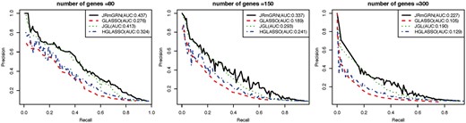
Precision-Recall curve of JRmGRN and three existing methods including graphical lasso (GLASSO), joint graphical lasso (JGL) and graphical lasso with hubs (HGLASSO) for Erdős-Rényi-based networks (Color version of this figure is available at Bioinformatics online.)

3.1.2 Results on Barabási-Albert (BA)-based network

BA-based network is used in Danaher et al. (2014) to evaluate the performance of network inferring algorithm. A big network consisted of a number of disconnected BA subnetwork. There are no explicit hub genes in these subnetworks; genes that have more high connectivity were considered hub genes. For a given number of tissues or conditions (⁠$\mathrm{K}$⁠), genes (⁠$\mathrm{p}$⁠), samples (⁠${\mathrm{n}}_{\mathrm{k}},\mathrm{ }\mathrm{k}\hspace{1em}=\hspace{1em}1,\dots ,\mathrm{ }\mathrm{K}$⁠), we used the following procedures to generate a BA-based network using corresponding gene expression data. (i) We divided $\mathrm{p}$ genes into m groups evenly. (ii) For each of first (1 –$\mathrm{ }\mathrm{\delta })\mathrm{m}$ gene groups, the BA-based subnetwork was the same across all $\mathrm{K}$ tissues or conditions and were generated with the function ‘barabasi.game’ from the R ‘igraph’ package. (iii) For each of the rest $\mathrm{\delta }\mathrm{m}$ gene groups, the BA-based subnetwork was different for each tissue or condition and were generated separately. (iv) For each edge in the network, we set the corresponding element in the precision matrix of the $\mathrm{k}$th tissue/condtion,$\mathrm{ }{\mathrm{\Theta }}^{\left(\mathrm{k}\right)}$⁠, to be a random number in $\left[-0.25,-0.75\right]\cup [0.25,\mathrm{ }0.75]$⁠. (v) We generated the gene expression of ${\mathrm{n}}_{\mathrm{k}}$ samples for the kth tissue or condition with ${\mathrm{n}}_{\mathrm{k}}$ independent multivariate normal distribution $\mathrm{N}(0,\mathrm{ }{{(\mathrm{\Theta }}^{\left(\mathrm{k}\right)})}^{-1})$⁠.

The simulation was conducted based on 2 tissues or conditions, 40 samples for each tissues or conditions and 8 subnetworks. The elementary network sparsity and hub sparsity were not explicitly implemented. We varied the parameters in the function ‘barabasi.game’ from R ‘igraph’ package to generate BA-based networks with desired elementary network sparsity (⁠$1-\mathrm{\alpha }$ = 0.98). We set seven out of eight subnetworks to be the same across two tissues or conditions, and one subnetwork to be different. We simulated 3 networks with 80, 160 and 320 genes, respectively.

The simulated BA gene network (Fig. 4A) and the estimated gene network (Fig. 4B) with 80 genes. JRmGRN successfully identified 191 edges with a true positive rate of 0.702, and falsely identified 290 edges with a false positive rate of 0.048. JRmGRN identified 17 genes as hub genes. The average number of edges connected to these 17 genes in the true network was 5.76, and the average number of edges connected to the rest 63 genes in true network are 3.05. Therefore, the hub genes identified by JRmGRN had much higher degree of connectivity. As pointed out in Han et al. (2004) and van den Heuvel and Sporns (2013), the genes with higher degrees of connectivity may be more important in biological development, which validates and manifests the usefulness of JRmGRN.

Fig. 4.

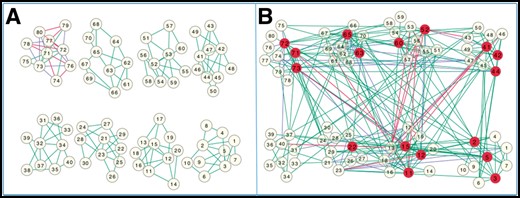
The simulated Barabási-Albert gene network (A) and the estimated gene network (B). In both A and B, the blue edges, the red edges and the green edges represent the edges from Tissues1-specific edges, Tissue2-specific edges and common edges from both tissues, respectively. The hub genes are highlighted in red in B (Color version of this figure is available at Bioinformatics online.)

The comparison of PR curves of JRmGRN and other methods are shown in Figure 5. When the number of genes were 80 or less, JRmGRN and JGL had similar performance, and they were better than the other two methods. As the number of genes increased, the performance of JRmGRN surpassed that of JGL and became the best.

Fig. 5.

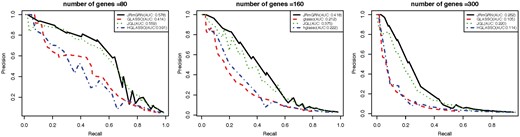
Precision-Recall curves of JRmGRN and three other existing methods including graphical lasso (GLASSO), joint graphical lasso (JGL) and graphical lasso with hubs (HGLASSO) on the Barabási-Albert-based network (Color version of this figure is available at Bioinformatics online.)

3.2 Results from real RNA-seq data of Arabidopsis thaliana

The Arabidopsis gene expression data used in this study are RNA-seq data generated from cotyledon tissue of Arabidopsis seedlings under two light regime conditions: low and high red: far-red (R: FR). There are 12 samples in each condition, with 2 replicates for each time point of 0.5, 1, 2, 3, 4 and 7 h. The SRA format data were downloaded through the accession identifier ‘GSE59722’ in the NCBI Gene Expression Omnibus (GEO) (http://www.ncbi.nlm. nih.gov/geo/). We first used the Rsubread software package (Liao et al., 2013) to transform the raw sequence reads to a matrix of raw counts, and then used the edgeR quasi-likelihood pipeline (Robinson et al., 2010) to obtain differentially expressed genes (DEGs) following the procedure given by Chen et al. (2016). There are 321 light related DEGs, as shown in Supplementary File 2. The Blom transform method (Zwiener et al., 2014) was used to transform the read counts data. The Blom transformation is a rank-based transformation, which back-transforms the uniformly distributed ranks to a standard normal distribution, i.e.

$${\mathrm{x}}_{\mathrm{i}\mathrm{j}}^{\mathrm{b}\mathrm{l}\mathrm{o}\mathrm{m}}={\mathrm{\varphi }}^{-1}\left(\frac{{\mathrm{r}\mathrm{a}\mathrm{n}\mathrm{k}}_{\mathrm{i}=1,\dots ,\mathrm{n}}\left({\mathrm{x}}_{\mathrm{i}\mathrm{j}}\right)-\mathrm{c}}{\mathrm{n}-2\mathrm{c}+1}\right)$$

with c = 3/8 and $\mathrm{\varphi }$ is the standardized cumulative distribution function.

The networks built based on the above method are shown in Figure 6. The common network of both low and high R and FR conditions is represented by the green edges with the 15 common hub genes being highlighted in yellow. All of these common hub genes had a connectivity > 172, which is at least 5 times larger than that of any the non-hub gene. Among these 15 hub genes, 8 were up-regulated in overall trends (BZO2H3, CCL, TCP11, PLPC5, AT1G62310, AT3G15570, NAC102 and AT3G45260) light-responsive. PLPC encodes a blue light receptor protein while BLH10 while 7 were down regulated in overall trends (BLH10, ELIP1, PD1, PEX11B, PLIM2a, WAV2 and POP12) upon low and high R and FR treatments. At least 8 genes, including PLPC, BEL10, CCL, PD1, ELIP1, PEX11B, AT3G15570, POP1 and WAV2, were previously reported to be encodes a protein that interacts with PLPC (PAS/LOV PROTEIN). Their interaction diminishes by blue light (Ogura et al., 2008). PD1 encodes a plastid-localized arogenate dehydratase required for blue light-induced production of phenylalanine (Warpeha et al., 2007) while PEX11B is involved in light response (Hu and Desai, 2008). ELIP1 is light-responsive (Rus Alvarez-Canterbury et al., 2014) and plays an essential role in the assembly or stabilization of photosynthetic pigment-protein complexes (Beck et al., 2017). CCL’s transcripts are differentially regulated at the level of mRNA stability at different times of day controlled by a circadian clock (Lidder et al., 2005). AT3G15570 encodes a phototropic-responsive NPH3 family protein. POP1 encodes a member of the NAP subfamily of ABC transporters whose expression pattern is regulated by light and sucrose (Marin et al., 2006). WAV2 negatively regulates root bending when roots alter their growth direction in response to environmental stimuli such as light (Mochizuki et al., 2005).

Fig. 6.

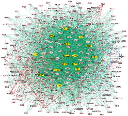
The gene regulatory networks built with JRmGRN. The blue and green edges represent the network built with the data from low red: far light regime condition while the red and green edges represent the network built with the data from high red: far light regime condition. The green edges represent common edges of the two networks (Color version of this figure is available at Bioinformatics online.)

4 Discussion

The results from synthetic data, which were generated with ER-based network or the BA-based network, clearly showed that JRmGRN outperformed several other methods, including GLASSO, HGLASSO and JGL for the reconstructing GRNs. Since common hub genes were explicitly modeled in the ER-based network, it was not surprised to see that JRmGRN had a higher accuracy in identifying common hub genes and had the largest area under the PR curves when the synthetic dataset from the ER-based network was used in the evaluation. In contrary, common hub genes were not clearly modeled though genes that had high connectivity can be seen in the BA-based network. When the synthetic dataset from the BA-based network was used in the evaluation, JRmGRN and JGL had similar performance as a small number of genes was included, whereas JRmGRN had a much better performance than JGL as a large number of genes was used.

When JRmGRN was used to construct gene networks using real gene expression dataset generated from Arabidopsis cotyledons under low to high red: far-red light regime conditions, it successfully built three networks and identified 15 common hub genes, and at least 9 of them were explicitly documented in existing literature for their involvement in light-response or related biological processes. Some of them, like ELIP1, PLPC and BLH10, play important roles in light perception and harvest in photosynthesis. In addition to these common hub genes, some other genes like bHLH071, a blue-light regulated gene (Jiao et al., 2003), and RSM1, a light-responsive gene (Soitamo et al., 2008), are identified to be hubs in low and high R: FR- specific networks, respectively, indicating the usefulness of the method in building two or more condition-specific networks and a common network across all conditions. We also implemented other three methods to the real dataset from Arabidopsis under far-red light and shade condition. We found JRmGRN and JGL identified much more numbers of common edges and less number of condition-specific edges than GLASSO and HGLASSO. HGLASSO identified 37 hub genes, 14 red: far-red-specific and 23 shade-specific hub genes. Of these 37 hub genes, TCP11, PD1 PLIM2A and AT3G45260 are among the 15 hub genes of JRmGRN. Among the 15 hub genes identified by JRmGRN, 9 are involved in light response and considered to be positive, whereas among 37 hub genes identified by HGLASSO, 8 genes are involved in light response and considered to be positive [Supplementary File 1 (S8, S9)]. It appears that JRmGRN is more efficient in recognizing positive hubs.

In the model of JRmGRN, four tuning parameters were used and a grid search was employed to find the optimal turning parameters, resulting in the optimal model based on the BIC like criterion. For a fixed set of tuning parameters, an efficient ADMM algorithm was derived and implemented to enable a fast estimation of precision matrices. Theoretical properties of the penalized likelihood function were also investigated and used to reduce the search space of tuning parameters. For a fixed set of tuning parameters, using a Mac desktop computer with 2.2 GHz Intel Core i7 processor and 16 GB 1600 MHz DDR3 memory, the average running times for estimating the precision matrices were about 30 s for 100 genes, 2.5 min for 200 genes, 6 min for 300 genes, 25 min for 500 genes and 3.7 h for 1000 genes, respectively. Therefore, implementation of JRmGRN allows us to reconstruct GRNs for 500 genes within a reasonable time frame by an ordinary desktop computer. In future, we will explore two possible strategies to reduce the computational burden so that JRmGRN can be used for a large number of genes. First, instead of using the grid search, we will investigate how the heuristic search algorithms, such the genetic algorithm (Grefenstette, 1987) and taboo (Glover, 1989; Glover, 1990) perform. Secondly, we will find out how the domain knowledge on gene networks and differentially expressed genes can be used to reduce the search space of tuning parameters.

In the current model of JRmGRN, it is assumed that all hub genes are shared across different tissues or conditions. In many situations, hub genes that are specific to an individual network also exist. One of our future works is to extend the current model to incorporate both common and unique hub genes. This can be done by adding an additional symmetric matrix to the decomposition of the precision matrix. The corresponding penalized log likelihood function and an efficient algorithm will be developed accordingly.

5 Conclusion

We proposed JRmGRN as a novel method for joint construction of GRNs using gene expression data from either several tissues or environmental conditions. The model was based on a convex penalized log likelihood function that not only took gene network sparsity and similarity into account but also explicitly modeled common hub genes across multiple GRNs, leading to multiple networks with common network moieties being highlighted. The resulting networks can significantly advance our understanding of genetic regulation of various biological processes. Reconstruction of both common moieties and each individual network corresponding to a tissue or a condition was improved by borrowing information of common hub genes and regulatory relationships from other individual networks. Therefore, JRmGRN can potentially generate more accurate gene networks, as manifested by the precision recall curves.

Funding

This work was supported by the Advances in Biological Informatics (ABI) National Science Foundation collaborative research grant awards DBI-1458130 to H.W., DBI-1458597 to P.X.Z. and DBI-1458515 to S.X. The funders had no roles in study design, data collection and analysis, decision to publish, or preparation of the manuscript.

Conflict of Interest: none declared.