


Abstract
Residue–residue contact prediction through direct coupling analysis has reached impressive accuracy, but yet higher accuracy will be needed to allow for routine modelling of protein structures. One way to improve the prediction accuracy is to filter predicted contacts using knowledge about the particular protein of interest or knowledge about protein structures in general.
We focus on the latter and discuss a set of filters that can be used to remove false positive contact predictions. Each filter depends on one or a few cut-off parameters for which the filter performance was investigated. Combining all filters while using default parameters resulted for a test set of 851 protein domains in the removal of 29% of the predictions of which 92% were indeed false positives.
All data and scripts are available at http://comprec-lin.iiar.pwr.edu.pl/FPfilter/.
Supplementary data are available at Bioinformatics online.
1 Introduction
Knowledge about the three-dimensional (3D) structure of proteins is essential for many types of research in the life sciences. Despite recent technology breakthroughs, it is still a major task to experimentally determine the structure of a protein, and consequently many methods have been devised to predict them in silico. Homology modelling is the method of choice when the structure of a homologous protein (the so-called template) is available. When no template can be found, one has to resort to more indirect methods like the prediction of residue–residue contacts followed by structure reconstruction techniques reminiscent of what is used in the NMR community (e.g. Bohr et al., 1993; Konopka et al., 2014; Saitoh et al., 1993; Skolnick et al., 1997; Vendruscolo et al., 1997). It has been often suggested (e.g. Altschuh et al., 1988; Dunn et al., 2008; Fariselli et al., 2001; Göbel et al., 1994; Morcos et al., 2011; Neher, 1994; Pollock and Taylor, 1997; Shindyalov et al., 1994; Weigt et al., 2009) that correlated mutations in multiple sequence alignments (MSAs) are indicative of residue–residue contacts because if two residues make a contact in the structure and one of them mutates, the other one should mutate too, to compensate. Residue pairs that are in contact thus tend to either stay conserved together or mutate together (Marks et al., 2011; Morcos et al., 2011). The importance of this methodology is exemplified by the fact that the CASP experiment (Moult et al., 1995, 2016) has a special section dedicated to contact prediction (Monastyrskyy et al., 2016). Today’s best methods are based on direct coupling analysis (DCA) of correlated mutations that are based on either the Potts model (e.g. Cocco et al., 2013; Ekeberg et al., 2013; Feinauer et al., 2014; Morcos et al., 2011; Skwark et al., 2013; Zhang et al., 2016) or other approaches, such as the sparse inverse covariance estimation as in PSICOV (Jones et al., 2012). For brevity, from here on, we will call all these methods as ‘DCA methods’. The quality of DCA methods so far typically has been around 40% true positives (TP) for the 100 strongest predicted contacts. When joined with predictions of other sequence features the TP rate can get significantly higher (Jones et al., 2015; Wang et al., 2017a), but still not high enough for routine 3D modelling of protein structures. Nevertheless, contact predictions have successfully guided transmembrane protein structures prediction (Hopf et al., 2012; Wang and Barth, 2015; Wang et al., 2017a), RNA secondary structure prediction (De Leonardis et al., 2015), protein–protein interaction prediction (Guo et al., 2015; Hopf et al., 2014; Horn et al., 1998; Iserte et al., 2015; Ovchinnikov et al., 2014) and even modelling of completely unknown protein folds (Ovchinnikov et al., 2017).
Several studies illustrated that the use of additional knowledge about the molecule of interest allows for better use of DCA results. Marks et al., for example, reconstructed the 3D structure of 15 proteins representing different fold classes using contacts predicted with their mean-field DCA—EVfold software and extensive manual inspection of the MSAs, the predicted contacts and a large number of possible structure models (Marks et al., 2011). Hopf et al. examined 25 membrane proteins and showed that manual inspection of contacts and removal of those that were inconsistent with the transmembrane topology was instrumental for the success (Hopf et al., 2012). Gouldson et al. used correlated mutations to determine the dimerization mode of G protein-coupled receptors (Gouldson et al., 2001). Hopf et al. used this same idea in reverse to improve the structure prediction by elimination of residue pairs that were related because of oligomeric interactions rather than intra-monomer contacts (Hopf et al., 2012). The importance of removal of inter-monomer contacts has been alluded to in many articles (e.g. Hopf et al., 2012, 2014; Kosciolek and Jones, 2014; Marks et al., 2011; Ovchinnikov et al., 2014).
We introduce a series of filters that allow for the accurate removal of false positives (FP) from the set of predicted contacts. These filters use knowledge about protein structures in general, and about the evolution of protein sequences and structures. We remove contacts between residues in the same secondary structure element and between the two beginnings and between the two ends of sequence-adjacent secondary structure elements. DCA-based methods have difficulties separating intra- from inter-molecular contacts. Because many proteins dimerize using their N- and C-terminal ends, we remove contacts between them. Contacts between solvent accessible residues and buried residues are rare. We therefore remove contacts between residues with a large difference in their predicted solvent accessibility. One of the main causes for occurrence of FP in the prediction is that correlated mutations are more often related to the functional importance of residues than to their structural relevance (Hopf et al., 2012, 2017; Oliveira et al., 2003). Contacts that are related to functional aspects (associated with ligand binding) and not directly to protein structure aspects often consist of residues that are highly conserved in the MSA (Oliveira et al., 2003; Reva et al., 2007). We therefore also filter contacts based on aspects of the MSA such as sequence entropy and the fraction of gaps.
We investigated how the performance of the filters relates to cut-off parameters by analyzing the number of filtered contacts, the filter accuracy and the increase of the TP rate. When all our filters are used with default parameters, 29% of the contacts are removed. About 92% of the removed contacts are FPs, which led to an increase of the average TP rate from 22% to 26% for the 851 proteins in our test set.
2 Materials and methods
2.1 Dataset
Filters were optimized using the training set that consists of the 804 protein chains used by the gplmDCA authors to test their method (Feinauer et al., 2014). This list of chains, together with their PDB files, gplmDCA scores and MSA files used to run gplmDCA is available online at http://gplmdca.aurell.org/input-data.
The filters were tested using a group of domains selected from SCOP (Murzin et al., 1995) that were used in an earlier work (Wozniak et al., 2017b). These domains have no alternate side-chain conformations, no missing residues inside the domain and contain only the 20 canonical amino acid types. All domains that were structurally similar to any of the chains in the training set (TM score 0.7 or higher) were removed (Zhang and Skolnick, 2005). The final test set contained 851 domains.
2.2 Contact definition
Two residues are called in contact when they are separated in the sequence by more than four residue positions and their Cβ atoms are not farther from each other than 8 Å.
2.3 Selection of strongest predicted contacts
Residue pairs were sorted in descending order of gplmDCA score (DS). We denote the top N pairs as the ‘strongest predicted contacts’. N = 20, 50, 100, 200, L/2, L and 3L/2 were used, in which L is the length of the target sequence.
2.4 Secondary structure and solvent accessibility prediction
Secondary structures and relative solvent accessibilities (RSA) were predicted with SSpro and ACCpro20, respectively. These methods are a part of the SCRATCH 5.2 software package (Magnan and Baldi, 2014). The get_abinitio_predictions script was used to ensure that homologous structures are not used by the software. This script is also provided in the SCRATCH package.
2.5 Filters
We introduce seven filters (A–G). Filters A and B use knowledge about the relation between sequence evolution and protein structure. Filters C–F use knowledge about the relative location of residues in the structure (like residues at the beginning of a helix cannot contact residues at the end of that same helix). Filter G uses the difference in (predicted) solvent accessibility between the two residues in a contact pair.
- A. Low entropy contacts. This filter removes contacts when at least one residue has a Shannon entropy H in the MSA below the cut-off Tent. H at sequence position k in the MSA is given by:in which f(ik) is the frequency of amino acid type i at sequence position k. The gap is treated as the 21st residue type. We examined the effect of Tent values between 0.02 and 0.9.(1)
B. Frequent gap contacts. Contacts are removed when at least one residue position in the MSA has a percentage of gaps greater than Tgaps. We examined the effect of Tgaps between 5% and 95%.
C. Intra-secondary structure contacts. Contacts are removed when the residues are located in the same regular secondary structure element (alpha helix or beta strand) and have a sequence separation larger than Sintra. We examined the effect of Sintra between 5 and 16.
D. Inter-secondary structure contacts. Contacts are removed when both residues are at the beginning or both are at the end of two regular secondary structure elements that are adjacent in the sequence. The following parameters were introduced (values examined are given in brackets):
Sinter: minimal separation between residues predicted to make a contact (5–16)
Sloop: maximal separation between two sequence-adjacent regular secondary structure elements (1–8)
Both residues must be located within e positions from the end of the secondary structure element (1–6)
- E. Inter-terminus contacts. Contacts are removed when their normalized sequence separation Snorm is higher than Snt. Snorm for residues at positions i and j is given by:in which L is the protein sequence length. We examined the effect of Snt between 0.2 and 0.95.(2)
F. Terminus contacts. Contacts are removed when at least one residue is among either the first t, or among the last t residues in the chain, and when both residues have their RSA higher than TRSA. We examined the effect of t between 1 and 20, and TRSA between 5 and 90.
- G. Buried-exposed contacts. Contacts between residues at positions i and j are removed when the difference between their RSAs, RSAdiff, matches:in which DSi,j is the gplmDCA score for the contact between residues at positions i and j. We examined the effect of a between −10 and 55, and of b between 0 and 140.(3)
Three filters that were described previously by Marks et al. (2011) were implemented to provide a point of reference:
A. Secondary structure straddling contacts are contacts between residues that are both close to or inside the same regular secondary structure element (alpha helix, H; beta strand, E). Following Marks et al. contacts were forecasted to be FP when:
⟨Hs-3; He⟩
[Hs-1; He+1]
⟨Es-4; Ee⟩
[Es-1; Ee+1]
[Es-2; Ee+2] (for strand of at least five residue length)
⟨a, b⟩ are contacts between residues at positions i and j in which i≥ a, i ≤ b, j ≥a and j ≤b
[a, b] are contacts between residues at positions i and j in which i = a and j = b
Hs is the position of the first residue in an alpha helix
He is the position of the last residue in an alpha helix
Es is the position of the first residue in a beta strand
Ee is the position of the last residue in a beta strand
B. Highly conserved contacts include one residue that is more than 95% conserved in the MSA. Cys–Cys pairs are treated separately.
C. The non-strongest Cys–Cys contact. For each cysteine, only its highest scored Cys–Cys pair is allowed from the top N predicted contacts.
2.6 Filter evaluation
The list of predicted contacts contains TP and FP. When we remove contacts, we can thus either remove a TP (which we will call a TPr), or remove a FP (which we will call a FPr). Three scores are used to assess the filter performance:
- A. The filter accuracy value (FAV) describes the quality of the filter. If a filter removes X predicted from the list, and Y% of these X contacts indeed were FP, and thus correctly removed, then the FAV score is Y. An ideal filter would yield Y = 100%. A bad filter has the FAV score lower than the FP rate.in which(4)
FPr is the number of removed FP contacts
TPr is the number of removed TP contacts
Reported FAVs are always the average over the values calculated for proteins in the dataset, unless mentioned otherwise.
- B. The positive predictive value (PPV) is the percentage of correctly predicted contacts. The increase of PPV (PPVinc) is the improvement in prediction accuracy resulting from filtering. Obviously, the FAV score must be larger than the FP rate of the unfiltered prediction for any filter to result in a positive PPVinc. PPVinc is given in percentage points (pp).in which(5)
TPafter is the number of true positives among the predicted contacts after filtering
Pafter is the number of predicted contacts left after filtering
PPVori is the original PPV; before filtering
Reported PPVinc values are always the average of the PPVinc values of all proteins in the dataset.
C. Fraction of filtered-out contacts (FFO) is the percentage of predicted contacts that were removed.
2.7 Software
Results were analysed using Java 1.7 and MATLAB scripts. Predicted and filtered-out contacts were mapped on structures and visually inspected with YASARA (Krieger and Vriend, 2015). All data and scripts used to optimize and evaluate filters are available at http://comprec-lin.iiar.pwr.edu.pl/FPfilter/.
3 Results
We describe 10 filters, 3 of which were previously described by Marks et al. (2011) and 7 are introduced here. The seven new filters contain user-selectable parameters. These scores should be used differently when the emphasis is on precision than when it is on recall, and it will be discussed how to make these choices. We have selected default parameters for each filter to give it a FAV score close to 90% on our training set.
Each filter has between 1 and 3 parameters that the user can choose to influence the precision and recall. It is computationally intractable to work out how to combine all these parameters to optimally achieve the desired results. We will show how each of the 10 filters performs, and will address their additivity. Finally, we will test the performance of each filter on our test set using default parameters.
3.1 Low entropy filter
Residues with very low sequence entropy (H) in the MSA tend to be involved in the main function of the protein, while residues with intermediate H tend to participate in auxiliary functions and residues with very high H tend to not have any functional role (Oliveira et al., 2003). Therefore, if a predicted contact involves residues with very low H, it is more likely that the residues co-mutated to maintain a function and less likely to be a TP contact. The low entropy contact filter removes contacts in which at least one residue position k has Hk lower than the threshold Tent.
Figure 1A shows how FAV, FFO and PPVinc vary with the cut-off value Tent. When Tent increases from 0.0 till 0.3 the FFO increases while the FAV decreases. The average FP rate for the training set is 71% so that PPVinc becomes negative once Tent has increased so much that the FAV falls below 71%, which happens around Tent = 0.4. Remarkably, PPVinc rises sharply when Tent increases beyond 0.7, but this is probably a spurious result as only very few predicted contacts are left. We set the default value for Tent at 0.02 resulting in FAV = 93%, FFO = 0.4% and PPVinc = 0.05 pp.
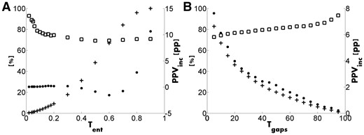
Results of (A) the low entropy filter and (B) the frequent gap filter. FAV (squares) and FFO (crosses) are percentages (left ordinate), while PPVinc (dots) is in pp (right ordinate)
3.2 Frequent gap filter
The quality of DCA predictions critically depends on the quality of the MSA, and the latter is likely lower at positions where many gaps are observed. The parameter Tgaps determines how many gaps are maximally allowed to occur at any sequence position in the MSA. Figure 1B shows the results for this filter for Tgaps ranging from 5 to 95. This figure illustrates beautifully the problem of parameter selection in relation to precision and recall. When Tgaps goes from 5 to 95, the FFO continuously decreases while the FAV increases (and PPVinc thus decreases too). We set the default value for Tgaps at 95% resulting in FAV = 93%, FFO = 1.2% and PPVinc = 0.2 pp.
3.3 Intra-secondary structure filter
The intra-secondary structure filter removes contacts in which both residues are in the same regular secondary structure element (α-helix or β-strand) and are separated by more than a certain number (Sintra) of residues. This filter was designed mainly to remove contacts between corresponding secondary structure elements that contact each other inter-molecularly in a homo-dimer. DCA methods often predict such contacts as intra-molecular contacts. When the 3D structure gets constructed using these contacts, the secondary structure element will bend in a very unnatural way (e.g. Nabuurs et al., 2006; Wozniak et al., 2017a). Figure 2A shows how FAV, FFO and PPVinc depend on Sintra. Obviously, a higher Sintra results in a lower number of filtered contacts (see Fig. 2A), and a lower influence on PPVinc. The FAV value is higher than 95% for any value of Sintra, so we set its default at 5 residues achieving FAV = 95%, FFO = 5.9% and PPVinc=1.2 pp. Sintra shorter than 5 makes no sense as contacts between residues with such a short sequence separation are never predicted, anyway.
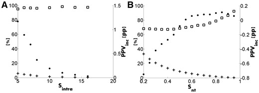
Results of (A) the intra-secondary structure filter and (B) the inter-terminus filter. FAV (squares) and FFO (crosses) are percentages (left ordinate), while PPVinc (dots) is in pp (right ordinate)
The performance of the intra-secondary structure contact filter depends on the secondary structure prediction accuracy. We investigated this accuracy by repeating the study with secondary structures determined with DSSP instead of the SSpro predicted ones. This increased the FAV value from 95% to almost 99% for N = 200 and Sintra = 5, which shows that this filter will become more accurate when better secondary structure prediction software will, in due time, become available.
3.4 Inter-terminus filter
The inter-terminus filter removes contacts between residues that are separated by a normalized sequence separation (Snorm) higher than the Snt cut-off parameter. This filter was designed because we realized that contacts between the N- and C-terminus were far more often inter-molecular than intra-molecular. Figure 3 shows original PPV of gplmDCA for various combinations of the Snorm and the gplmDCA score (DS). Figure 3 shows that most PPVs are low (blue squares) when Snorm is above 0.9.
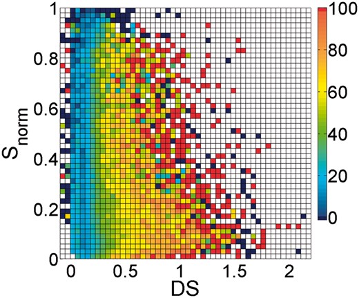
PPV as a function of the gplmDCA score (DS) and the normalized sequence separation (Snorm). The colours relate to the PPV as indicated in the colour-bar at the right-hand side. Red squares represent a PPV of 100%. White squares indicate no data (Color version of this figure is available at Bioinformatics online.)
Figure 2B shows the relation between FAV, FFO and PPVinc for Snt values between 0.2 and 0.95. Obviously, the higher Snt the lower FFO, and for Snt = 0.95 FFO is only 0.3%. On the other hand, the higher Snt, the higher will be FAV and PPVinc. Although the FAV value is maximal for Snt = 0.95, the highest value of PPVinc is obtained for Snt = 0.85. The PPVinc values, though, differ only marginally between Snt = 0.95 and Snt = 0.85 (0.09 pp and 0.11 pp, respectively). Therefore, we chose as default Snt = 0.95, which leads to FAV = 92.3%, FFO = 0.3% and PPVinc = 0.09 pp, respectively.
Figure 2B shows that it is good for PPVinc to remove all contacts predicted between residues that are separated from each other by at least 60% of the sequence length. In a separate experiment, we observed that (long range) contacts between Pfam domains (Finn et al., 2016) in the same protein are predicted with slightly lower accuracy than short-range contacts in the same protein. This is very disappointing because it is known from the field of NMR structure determination that long-range contacts are much more important for 3D structure determination than the short-range ones (Nabuurs et al., 2003).
3.5 Inter-secondary structure filter
The inter-secondary structure filter removes contacts between residues at both beginnings or at both ends of two adjacent regular secondary structure elements. This filter is based on the observation that 85% of all pairs of sequence-adjacent elements pack anti-parallel more than parallel. For these 85%, contacts between either their N-termini or C-termini are highly unlikely (see Supplementary Fig. S1—Others). We introduced three parameters: Sinter is the minimal sequence separation between the contacting residues; Sloop is the maximal sequence separation between the two sequence-adjacent regular secondary structure elements (loop length); e is the sequence distance of the residue to the relevant end of its regular secondary structure element. Each of these three parameters can have a series of values (see Section 2), together resulting in 552 combinations. For all 552 combinations, the values of FAV, FFO and PPVinc are provided in the Supplementary Material—Parameters Evaluation. Obviously, the lower the values of Sloop and e, and the greater the value of Sinter, the more likely it is that the predicted contact should be removed. It is very difficult to represent the 552 parameter combinations graphically. We therefore provide some examples of parameter combinations and their results in Table 1.
Selected parameter combinations for the inter-secondary structure filter and the resulting FAV, FFO and PPVinc values
| Sinter | Sloop | e | FAV | PPVinc | FFO |
|---|---|---|---|---|---|
| 6 | 3 | 5 | 69.95 | −0.104 | 2.421 |
| 16 | 6 | 6 | 68.24 | 0 | 1.066 |
| 6 | 2 | 6 | 76.67 | 0.08 | 1.687 |
| 6 | 1 | 2 | 91.95 | 0.016 | 0.089 |
| 16 | 1 | 1 | 100.0 | 0.002 | 0.002 |
| 6 | 1 | 6 | 84.37 | 0.086 | 0.723 |
| Sinter | Sloop | e | FAV | PPVinc | FFO |
|---|---|---|---|---|---|
| 6 | 3 | 5 | 69.95 | −0.104 | 2.421 |
| 16 | 6 | 6 | 68.24 | 0 | 1.066 |
| 6 | 2 | 6 | 76.67 | 0.08 | 1.687 |
| 6 | 1 | 2 | 91.95 | 0.016 | 0.089 |
| 16 | 1 | 1 | 100.0 | 0.002 | 0.002 |
| 6 | 1 | 6 | 84.37 | 0.086 | 0.723 |
Note: The values in the bottom row (Sinter = 6, Sloop = 1 and e = 6) were chosen as default values for this filter.
3.6 Terminus filter
The terminus filter removes contacts in which at least one residue is either near the N- or the C-terminus of the protein. The idea behind this filter is that N- and C-terminal residues are very often at the surface of the protein, which makes it unlikely that they are in contact with many other residues. Many contacts that are removed by this filter are also removed by the inter-terminus filter, which is presented in the later sections. This filter uses two parameters: the maximal sequence distance t to either of the two termini, and TRSA, which is the maximal RSA of the two residues. The accessibility constraint was introduced to prevent that contacts are removed with terminal residues that are not very exposed. Figure 4A shows that predicted contacts are more likely to be TP when their residues are buried.
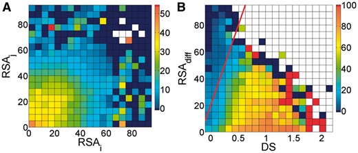
(A) PPV of gplmDCA as a function of the RSA values of the contact pairs (i, j). The colours relate to the PPV as indicated in the colour-bar at the right-hand side. Dark blue squares represent a PPV of 0.0%. White squares indicate no data. (B) PPV of gplmDCA as function of the difference between the RSAs of the two residues (RSAdiff) and the gplmDCA score (DS). The red line represents RSAdiff = 20 + 120·DS. All contacts that are to the top left of this red line were removed. The colours relate to the PPV as indicated in the colour-bar at the right-hand side. Red squares represent a PPV of 100.0%. White squares indicate no data (Color version of this figure is available at Bioinformatics online.)
Figure 5 shows the performance of the terminus filter for t ranging from 1 till 20 and TRSA ranging from 5 till 90. Figure 5 makes clear that the relation between TRSA and the results is rather independent of t. We therefore chose as defaults TRSA = 35 and t = 15 which leads to FAV = 90.1%, FFO = 5.3% and PPVinc = 0.7 pp.
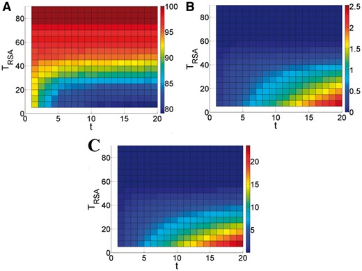
FAV (A), PPVinc (B) and FFO (C) of the terminus filter for combinations of maximal RSA (TRSA) and maximal sequence distance from the N-termini or C-termini (t). For each of the three figures, the relation between colour and resulting filter evaluation score is given in the colour bar to the right of the plot (Color version of this figure is available at Bioinformatics online.)
3.7 Buried-exposed filter
We realized that contacts between buried and solvent accessible residues are rare, and Figure 4B indeed shows that predicted contacts tend to be FP when the difference between the RSA of the two residues is larger than about 50. It should be noted that the squares in Figure 4B can represent radically different numbers of contacts. Some of the squares near the bottom left corner represent more than 10 000 contacts, while most squares near the white area represent only 1 till 10 contacts. We decided to draw the line RSAdiff = a + b·DS (see Section 2) and remove all contacts that are to the top left of this line. It is difficult to graphically represent the results of such a multi-parameter function. We exhaustively list the results in the Supplementary Material——Parameters Evaluation. We choose a = 20 and b = 120 as defaults, which resulted in FAV = 91.4%, FFO = 8.9% and PPVinc = 1.35 pp.
3.8 Filters introduced by Marks et al.
In their seminal paper of 2011, Marks et al. introduced the idea of filtering contacts predicted by DCA. We implemented their methods exactly as described, and applied them to our standard 804 protein training set to create a point of reference. Marks’ secondary structure straddling filter works very similar to our intra-secondary structure filter, and all contacts removed by the intra-secondary structure filter are also included in the set of contacts removed by the straddling filter. Supplementary Table S1—Others shows the results of the straddling filter compared with the intra-secondary structure filter with parameters that produce the most similar FAV.
We noticed that using secondary structure assignments derived from DSSP rather than predicted ones (that are always available, of course) improved the intra-secondary structure filter’s FAV performance a lot. We do not observe this same effect for the straddling filter for which the FAV increases only from 83.9% to 84.3% for N = 200 when DSSP is used instead of a predicted secondary structure.
Marks et al. treat Cys–Cys contacts as an exception when filtering highly conserved contacts (Marks et al., 2011). This filter is based on the knowledge that cysteines can form a disulphide bond with only one other cysteine. It has FAV = 57% for N = 200. This filter actually causes worse PPVinc scores. Because of this low FAV, we did not implement a similar filter, but rather analysed how all our filters together (using default parameters) performed on the predicted Cys–Cys contacts in the training set. The results (shown in Supplementary Table S1 as Cys–Cys*) are actually even worse, but as all our filters together reject only few Cys–Cys contact pairs, the decrease of PPVinc is less. In total, our seven filters rejected 44 Cys–Cys pairs. The buried-exposed filter removed 8 of 11 contacts correctly, but the entropy filter removed only 7 of 27 correctly. It seems that predicted Cys–Cys contacts better are not filtered out.
3.9 Filter comparison
It is commonly known that the PPV is higher when fewer contacts are predicted. In Figure 6 we present the results for all 10 filters when used with default parameters for N = 20, 50, 100 and 200.
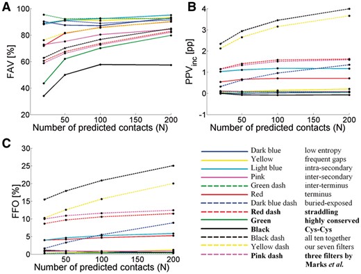
Results for N = 20, 50, 100 and 200 for each individual filter, for all 10 filters together, for our seven new filters together, and for the three filters from Marks et al. together. (A) FAV, (B) PPVinc, and (C) FFO. Note that the lines are for clarity only and that the ordinate of the FAV plot starts at 20. Filters introduced by Marks et al. are listed in bold (Color version of this figure is available at Bioinformatics online.)
The intra-secondary structure filter gives the best FAV, while all 10 filters together give both the highest FFO (obviously) and the highest PPVinc. The FAV of all 10 filters together is near the average of the 10 lines for filters separately. It is remarkable that the inter-terminus filter has a higher FAV at N = 20 than for any other value of N. Obviously, with N = 20, the number of predicted contacts is 10 times less than with N = 200, so the significance of this observation remains a point of doubt. Conclusions from Figure 6 are similar when N depends on the sequence length (see Supplementary Material—Default Parameters).
3.10 Filter intersection
Often, the same contact is removed by multiple filters. Therefore the FAV, FFO and PPVinc results do not add up linearly when filters are used together. Obviously, FFO will never diminish when more filters are used, but that is not necessarily the case too for FAV and PPVinc, albeit Figure 6B seems to suggest that they do a bit. Table 2 shows the intersection of contacts removed by the 10 filters. This table is not symmetrical with respect to the diagonal as the number of contacts removed by both filters is a different percentage of the total number rejected by each of those two filters individually.
Intersection of removed contacts between different filters
| A | B | C | D | E | F | G | H | I | J | |
|---|---|---|---|---|---|---|---|---|---|---|
| A | 100 | 3.7 | 6.4 | 65.1 | 19.7 | 27 | 3.1 | 18.8 | 0 | 5.5 |
| B | 0.6 | 100 | 0 | 0 | 0.5 | 0.6 | 1 | 1.6 | 0.3 | 2.1 |
| C | 7.2 | 0 | 100 | 0 | 1 | 3.2 | 7 | 7.8 | 0.3 | 51 |
| D | 3.8 | 0 | 0 | 100 | 8.7 | 8.2 | 0.9 | 8.1 | 0.3 | 0 |
| E | 1.8 | 0.3 | 0.1 | 13.3 | 100 | 28.7 | 3.1 | 25.4 | 3.1 | 0.1 |
| F | 6.3 | 0.8 | 0.7 | 32.5 | 73.6 | 100 | 6.2 | 59.8 | 0 | 0.8 |
| G | 5.3 | 9.8 | 10.7 | 25.7 | 58.8 | 44.9 | 100 | 20.7 | 1.4 | 11.3 |
| H | 1.9 | 1 | 0.7 | 14.3 | 29.1 | 26.7 | 1.3 | 100 | 0 | 0.6 |
| I | 0 | 0.1 | 0 | 0.4 | 3.1 | 0 | 0.1 | 0 | 100 | 0 |
| J | 12.1 | 26.2 | 100 | 0 | 3.5 | 7.3 | 14.6 | 12.5 | 1 | 100 |
Notes: Letters represent filters as indicated in the table. Values are the percentages of intersecting removed contacts relative to the total number of contacts removed by the filter of that column. So, 0.6% of all contacts removed by filter A were also removed by filter B, while 3.7% of the contacts removed by B are also removed by A. (A) terminus; (B) inter-secondary structure; (C) intra-secondary structure; (D) inter-terminus; (E) low entropy; (F) frequent gaps; (G) buried exposed; (H) highly conserved; (I) Cys–Cys; (J) secondary structure straddling.
For example, 0.6% of all contacts removed by the terminus filter (A in Table 2) were also removed by the inter-secondary filter (B in Table 2). On the other hand, 3.7% of the contacts removed by B were also removed by A. So, the overlap between filters A and B is rather small, and consequently, their results will be nearly perfectly additive.
The overlap between the intra-secondary structure filter (C) and the straddling filter (J) is highly asymmetric. This was expected as principally each contact removed by the former is also removed by the latter, but not vice versa (100% and 51%, respectively). A similar effect is observed between the low entropy (E) and frequent gaps (F) filters. Almost 74% of contacts removed by the former one were also removed by the latter. This is because a high number of gaps at an MSA position leads to a low entropy value. Similarly, about 65% of contacts removed by the inter-terminus filter (D) were also removed by the terminus filter (A). Except for the pairs of filters mentioned above, our filters are based on strongly different concepts, and if a contact should be removed by one filter but not by another, it will still be removed. That is why our filters can be used additively and their parameters optimized independently. A machine learning method that optimizes all parameters for all filters together will undoubtedly lead to higher FAV, FFO and PPVinc scores. Unfortunately, this is rather big task that at present seems computationally intractable. Also, the clarity of our bio-knowledge-based rules would then get lost as happens so often with ‘black box-like’ methods.
3.11 Filter performance as a function of prediction accuracy
We wondered if the performance of the filters could be a function of the quality of the contact predictions. For this purpose, we sorted the training set by the PPVs of the gplmDCA prediction and split the list in four equally large groups. The influence of the parameters on the filter performance is very similar among the four groups (the lists of these four groups are available online).
We noticed that the FAV of a filter must be higher than the FP rate of the contact prediction for a particular protein to increase this PPV. For example, to increase a PPV of 10% (i.e. FP rate = 90%), the FAV value must be higher than 90%, but when the prediction is better and the PPV is 30%, then the FAV needs to be no higher than 70%. This might feel counter-intuitive because it means that it is easier to improve good predictions than bad ones.
Figure 7 shows the relation between PPVinc and FAV for the terminus filter for the worst and the best predicted group. The well predicted group has an average PPV of 57%, and the PPVinc is always positive when the FAV value is higher than about 55%. The PPV of the poorly predicted proteins ranges from 0% till 13%. To get their PPVinc more often positive then not a FAV higher than 93% is needed.
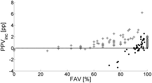
PPVinc and FAV for individual proteins when using the terminus filter. Black dots: proteins with PPV between 0% and 13%; grey crosses: proteins with PPV between 42.5% and 100%. Each dot represents one protein
3.12 Testing filter performance for default parameters
To prove that our default parameters do not work only for our training set, we tested the performance of all 10 filters using default parameters on our test set (see Section 2). The results are presented in Supplementary Tables S4 and S5—Default Parameters. For all values of N the FAV, PPVinc, and FFO are similar to those obtained for the training set. The dependence of the scores on N is also similar for the training set and the test set (Supplementary Tables S2 and S3—Default Parameters).
For N = 200, our seven filters together obtained FAV = 91.5%, FFO = 29% and PPVinc = 4 pp for the test set which actually is even a bit better than what was obtained for the training set (FAV = 90.3%, FFO = 20% and PPVinc=3.7 pp). More contacts were removed from the test set than from the training set, which seems related to the lower average PPV of gplmDCA for the SCOP domains than was obtained for the PDB chains in the training set (22% and 29%, respectively).
4 Discussion
Supplementary Figure S2—Others shows the relation between PPVinc and FAV for all 804 proteins in the training set, using all 10 filters with default parameters. The average PPVinc is 4.0 ± 3.9 pp, indicating that the filters improve the prediction quality in 92% of all cases. For the test set the average PPVinc was 3.9 ± 4.3 pp and prediction was improved for 86% of all cases.
We manually inspected the five proteins in our training set for which our seven filters produced the worst PPVinc when using default parameters. PDB file 1BH4 is a protein of only 30 amino acids for which the MSA contained only 262 sequences. The Cys–Cys filter removes 11 predicted contacts of which 10 are actually TP. The MSA for PDB file 3N1G holds 65 522 sequences, which is the maximum number HHblits (Remmert et al., 2012) can deal with. The alignment has a staggering 70% gaps, and it is thus not a surprise that the highly conserved filter and the gaps filter perform poorly. 1GPS is again a very small protein of only 47 residues. Its N- and C-terminal residues are in contact, which is very rare in structures in the PDB, and is always removed by the filters. The Cys–Cys filter and the conserved residue filter performed poorly on this molecule too. 1GPS also has a highly uncommon amino acid distribution with one side of the protein consisting of only arginines. 1FRA is a small protein with only 62 residues. Its Ramachandran plot looks very poor. 2E7S consists of one long helix, and all 200 predicted contacts were wrong (and all were removed by the filters).
These five examples illustrate an important point. The filters work well for middle-of-the-road proteins, but neither do they cope well with exceptional structure features, nor with predictions based on poor alignments. With each prediction, one should think about constraints set by the particular protein at hand. Hopf et al. (2012) realized that upon predicting transmembrane helix bundles one can blindly remove predicted contacts between residues expected to be located at opposite sides of the membrane. We implemented their filter and used it on the same 25 proteins they analysed. This removed 178 contacts (3.6%) of all predicted contacts with 90% accuracy. Out of these 178 contacts, only about 28 (16%) were also removed by any of our seven filters, which, by the way, presented a great performance in this case achieving FAV = 93%, FFO = 23% and PPVinc=6.6 pp. This means that our very generally applicable filters and the molecular class specific filters used by Hopf et al. work nicely additively.
One may device many more filters appropriate for a particular molecular class. The inter-terminus filter should be switched off for cyclical proteins, and no filter will work well for natively unfolded proteins. Also, the filters aimed at removing inter-molecular interactions perhaps should be used in reverse for amyloid proteins.
We introduced a set of filters that can, with high accuracy, remove FP-predicted contacts. The number of contacts removed by any filter depends strongly on which other filters had been applied before. When all 10 filters are used together, with default parameters, the number of removed contacts (expressed by FFO) becomes 25% with FAV = 85% and PPVinc = 4 pp for the training set. In Supplementary Tables S2 and S3 in —Default Parameters, we sum up the performance of each filter separately for the (default) parameters that we believe to lead to the best performance. Default parameters values are also listed in Supplementary Table S1.
The highest filter accuracy was obtained for the intra-secondary structure-related filter. The residues removed with this filter often have high DS value, because they often take part in functionally important inter-chain interactions in homo-oligomers. Contacts between the N- and C-terminus were removed using the inter-terminus filter. Such contacts are more often inter-molecular than intra-molecular. We applied the inter-terminus filter separately for monomeric and multimeric PDB files in our training set. We obtained FAV scores of 89.5% for monomers and 94.2% for the rest, as was expected. So, even though this filter was designed to remove dimer contacts, it works also reasonably well for monomers. The information about the oligomeric state of PDB files was obtained from PDBePISA (Krissinel and Henrick, 2007). We also tested the idea of filtering contacts predicted between different Pfam domains that are found in one protein of interest. This unfortunately led to a rather low FAV score of 63%. Because of that we abandoned this idea.
The FAV score of a filter must be higher than the FP rate of the contact prediction for any protein to increase its PPV. Obviously in the real life, when the protein structure is unknown, the PPV of a DCA method is not available. In such a case, PPV can be forecasted as described earlier (Wozniak et al., 2017b). The parameters of a selected filter can be then set using the data provided in the Supplementary Material—Parameters Evaluation to ensure a good FAV value and thus a positive value of PPVinc.
Recently, many methods have been developed that use so-called deep-learning techniques that is neural networks that use many hidden layers and often combine networks of different architecture. A good example is RaptorX (Wang et al., 2017a) that was one of the best methods in contact prediction during CASP11 (Monastyrskyy et al., 2016). RaptorX combines information about sequence conservation with predicted secondary structure, and solvent accessibility as input for a deep learning neural network. We tested the performance of our filters on contacts predicted with RaptorX using default parameters. The results for the test set are presented in Supplementary Table S6—Default Parameters for a series of values of N. RaptorX is typically used to predict the top N strongest predicted contacts with N equal L (the protein’s sequence length). For N = L, the PPV of RaptorX is 61% on our test set. Using our seven filters with default parameters resulted in FAV = 49%, PPVinc=0.3 pp and FFO = 5.8%. The highest FAV (84%) was achieved by the buried-exposed filter (see Supplementary Fig. S3—Others).
Overall, though, our filters work slightly worse for RaptorX than for gplmDCA. This is partially caused by the fact that only about 7% of all contacts filtered out from the gplmDCA results were also predicted with RaptorX; or in other words RaptorX works better than gplmDCA on our test set, so its results can be improved less. The RaptorX neural network uses information about secondary structure and solvent accessibility, which seems to automatically remove a large number of FP contacts that our filters remove from the gplmDCA results. Correspondingly, when RaptorX predicts more than L contacts, our filters work better (see Supplementary Table S6—Default Parameters), because the PPV of RaptorX decreases with the increase of N and our filters work better when more FP predictions are present (see Supplementary Fig. S4—Others). In summary, our filters can even improve the results from sophisticated methods such as deep neural networks.
We have shown that a series of filters, based on well-known facts about protein structures or MSAs, can improve the quality of DCA-based contact predictions. We are, unfortunately, still far away from predictions that are good enough to routinely predict 3D protein structures using techniques from the NMR field in which NMR measurements are replaced by DCA predictions. It is to be expected that filters based on knowledge that is applicable just to the one protein of interest can be used to further improve DCA predictions, but such knowledge is hard to implement in a generic fashion. Nevertheless, we can hope that fully automatic structure predictions will become routine, serving all those fields that rely on knowledge of the 3D structure of a protein.
Acknowledgements
Wroclaw Centre for Networking and Supercomputing at Wroclaw University of Science and Technology is acknowledged.
Funding
The work of P.P.W. and M.K. was supported by Statuary Funds. P.P.W acknowledges funding from the Polish National Science Centre (Etiuda 4, DEC-2016/20/T/NZ1/00514). The work of J.P. and M.S. was supported by Erasmus+ programme. G.V. acknowledges funding from the EU project NewProt (289350).
Conflict of Interest: none declared.
References

