Modelling BioNano optical data and simulation study of genome map assembly

Abstract

Motivation

The launch of the BioNano next-generation mapping system has greatly enhanced the performance of physical map construction, thus rapidly expanding the application of optical mapping in genome research. Data biases have profound implications for downstream applications. However, very little is known about the properties and biases of BioNano data, and the very factors that contribute to whole-genome optical map assembly.

Results

We generated BioNano molecule data from eight organisms with diverse base compositions. We first characterized the properties/biases of BioNano molecule data, i.e. molecule length distribution, false labelling signal, variation of optical resolution and coverage distribution bias, and their inducing factors such as chimeric molecules, fragile sites and DNA molecule stretching. Second, we developed the BioNano Molecule SIMulator (BMSIM), a novel computer simulation program for optical data. BMSIM, is of great use for future genome mapping projects. Third, we evaluated the experimental variables that impact whole-genome optical map assembly. Specifically, the effects of coverage depth, molecule length, false-positive and false-negative labelling signals, chimeric molecules and nicking enzyme and nick site density were investigated. Our simulation study provides the empirical findings on how to control experimental variables and gauge analytical parameters to maximize benefit and minimize cost on whole-genome optical map assembly.

Availability and implementation

BMSIM is freely available on: https://github.com/pingchen09990102/BMSIM.

Supplementary information

Supplementary data are available at Bioinformatics online.

1 Introduction

Genome physical mapping technologies have received increasing attention in recent years because of their ability to effectively complement the shortfalls of short-read sequencing technologies. Whereas the early physical mapping methods, such as OpGen optical mapping, were often expensive and labour intensive(Paux et al., 2008), the newly developed BioNano Irys system greatly enhances the throughput and performance of physical mapping by leveraging advances in nanoscale material engineering, fluorescent labelling of DNA molecules and imaging processing algorithms (Lam et al., 2012). BioNano optical mapping technology rapidly expanded its applications in many aspects of genome research, e.g. assessing and guiding sequence assembly (Chen et al., 2017; Zhihai et al., 2016), identification of satellite repeated sequences (Dong et al., 2016), resolving haplotypes (Pendleton et al., 2015) and the detection of structural variations (Cao et al., 2014).

As for popular sequencing technologies, data biases/errors are inevitable in the BioNano optical mapping system. BioNano optical mapping experiments are vulnerable to variations and perturbations of internal and external sources, creating data biases and variations that have profound implications for downstream applications. A non-random molecule distribution can hamper the haplotype resolution in regions of low coverage depth. Labelling errors on DNA molecules, i.e. BioNano molecules, can lead to false signals and incorrect variant calls. However, very little is known about the properties, biases and error rates of BioNano data or the factors that induce or contribute to them. The purpose of this study is threefold. First, it was designed to investigate the properties such as molecule length, false labelling signal, variation in optical resolution, coverage distribution bias and the data variations due to factors such as chimeric molecules, fragile sites and DNA molecule stretching, which have great impact on common applications of BioNano optical mapping technology. Based on our analyses, we developed statistical models to model the properties, biases and error profiles of BioNano molecule data and provided guidelines for filtering BioNano data to mitigate their impact on downstream applications. Second, we developed a novel optical data simulation program, BioNano Molecule SIMulator (BMSIM), for the generation of simulated BioNano molecule data. With available models, BMSIM can also be extended to simulate other optical mapping experiments. Third, we employed BMSIM to evaluate the impact of variable factors on the outcome of whole-genome optical map assembly. Specifically, the impacts of the coverage depth, molecule length, false signal rates, nicking enzyme and chimeric molecule were evaluated. We summarize the general rules for the design of whole-genome optical map projects and present guidelines for data processing and gauging the parameters for whole-genome optical map assembly.

2 Materials and methods

2.1 Data source and basic processing

We generated BioNano molecule data from eight organisms (Supplementary Table S1; and Supplementary Methods Section S1.1). Molecule data were then aligned and compared to their reference genomes, which were converted in silico into a restriction map according to the recognition signature of the nicking enzyme Nt.BspQI. Alignment was performed using RefAligner. Custom scripts (in Perl) were developed to process outputs from RefAligner and to extract information, e.g. aligning the positions of molecules and signals of labelling sites, etc. for further analysis. Statistical analysis and plotting were performed using R and MATLAB (R2016a).

2.2 Modelling the distribution of BioNano molecule length

To model the BioNano molecule length in the BioNano data simulator BMSIM, a molecule (with a size of $\iota$⁠) was first randomly selected from a distribution of molecules whose sizes are described by an exponential distribution $\iota \hspace{0.17em}\sim \hspace{0.17em}\hspace{0.17em}\text{exp}\hspace{0.17em}onential(\lambda )$ with the average size $\lambda$⁠. Next, the molecule with size $\iota$ was randomly sliced from one chromosome of the reference genome. If the molecule end exceeded the end of the chromosome, the shorter molecule was also retained.

2.3 Modelling for false-positive (FP) and false-negative (FN) labelling sites

It was reported (Valouev, 2006) that the false-positive sites resulting from random DNA nicks or the nonspecific action of endonuclease have no preference for regions of DNA molecules. Thus, the number of false positives, $R_{FP}$⁠, per fixed length of DNA (⁠$s$Kb), obeys a Poisson distribution with intensity parameter $\lambda$ (nick/Kb), i.e. $R_{FP}\sim Poisson(\lambda s)$⁠. The FPs were modelled as a homogeneous Poisson process with the rate $\lambda$ in BMSIM.

It was also reported (Das et al., 2010) that the labelling of each site is independent with an efficiency of p. Thus, the probability P of molecules with m sites labelled from a total of n sites observed is $\frac{n!}{m!(n-m)!}{P}^m{(1-P)}^{n-m}$⁠. Thus, whether true nick sites are labelled can be modelled as independent Bernoulli trials. Therefore, to model missing label events (FNs), we treated the nicking of each site as a Bernoulli event with the probability of success P in BMSIM.

2.4 Modelling for DNA molecule stretch variation in the BioNano system

DNA stretching is a complex interaction of several stochastic variables, such as the Brownian motion of DNA (Tegenfeldt et al., 2004), salt concentration (Jo et al., 2007) and flow voltage changes (Reccius et al., 2008), many of which have unknown distribution functions. It was reported (Chan, 2004) that the stretching of DNA molecules with free termini is not homogeneous. We devised the ‘stretch variation factor’ $R$ as a measurement of stretch variation for each DNA fragment between neighbouring sites in the BioNano system.

Stretch variation factor $R$ was defined as $R=le{n}_{measured}/le{n}_{reference}$⁠, where the reference length, $le{n}_{reference}$⁠, represents the number of DNA base between neighbouring sites, as obtained from the reference genome sequence aligned to the DNA fragment, and the measured length, $le{n}_{measured}$⁠, was computed for the DNA fragment between neighbouring sites by converting the pixels into a base number with a constant predefined for the Irys system (e.g. a constant of 500 bases per pixel, corresponding to 85% of the theoretical maximal DNA stretching; Lam et al., 2012; Shelton et al., 2015). According to the central-limit theorem (Dedecker, 1998), the distribution of the stretch variation factor $R$ for each region of DNA between neighbouring sites in the BioNano system was assumed to be Gaussian, $R\sim N(\mu ,{\sigma }^2)$⁠.

2.5 Modelling for the observed variation in optical resolution

Under ideal conditions, the likelihood of resolving two particles, $p_{resolving}$ was defined as a unit step function $H\left(x\right)$⁠:

$$H\left(x\right)=\{\begin{array}{l}0,x<t\\ 1,x>t\end{array}$$

which is a discontinuous function whose value is 0 when the distance between neighbouring sites $x$ is smaller than a resolution threshold $t$⁠, and 1 when the distance between neighbouring site $x$ is larger than a threshold $t$⁠.

However, we found that the optical resolution of the BioNano system is influenced by variations in the Irys machine conditions (e.g. temperature, flow-rate, emitted fluorescence light, vibration, sample density and sample/solution purity) and sample preparations (DNA quality, nicking and labelling reactions and fluorescent dye quality/quantity). The combined function of these variables led to the variation in optical resolution, which we observed when operating the BioNano system.

According to the Central Limit Theorem (Dedecker, 1998), the observed variation in optical resolution tends to have the effect of convolution with a Gaussian kernel. Under the net effect of convolving with a Gaussian kernel, the step function of the likelihood of resolving the neighbouring site $p_{resolving}$ was expected as a cumulative Gaussian kernel, i.e. the convolution of the unit step function $H\left(x\right)$ with a Gaussian function $G\left(x\right)$ (Broadbent, 1954; Hirschman and Vernon, 1955; Wang et al., 2005), which is defined as

where $x$ is the distance between two neighbouring sites, $G\left(v\right)$ is the Gaussian function $G\left(v\right)=\frac{1}{\sigma \sqrt{2\pi }}\text{exp}(-\frac{{(v-\mu )}^2}{2{\sigma }^2})$⁠. Model parameter estimation was based on non-linear regression using the curve fitting tool from MATLAB (R2016a). Model parameters were estimated with a mean of $\mu =1.2$⁠, and a standard deviation of $\sigma =0.9$⁠. Accordingly, two neighbouring sites 1.2 Kb apart have a 50% chance of being resolved, and two neighbouring sites 1.2 + 2 * 0.9 = 3 Kb apart have an approximately 97.5% probability of being resolved.

2.6 Modelling for fragile sites

A fragile site occurs when two nicking sites are located on opposite strands in close proximity. Its occurrence probability can be modelled as a function of the distance between two nicking sites on opposite strands. It should follow the exponential model that was previously used to estimate the breakage probability related to length (Griebel et al., 2012; Iyengar, 1981). The curve of the likelihood of breakage against the distance between nicking sites on opposite strands was found to fit that of exponential decay.

Therefore, the model of fragile site formation, i.e. the likelihood of breakage $p_{\text{breakage}}$ against the distance (dis) between nicking sites on opposite strands, was defined by the exponential model: $p_{\text{breakage}}=a*\hspace{0.17em}\text{exp}(b*\text{dis})$⁠, where dis is the distance between nicking sites on opposite strands, $a$ and $b$ are two empirical parameters (a = 0.7758, b = −0.006984) that are estimated from empirical data using cftool. In simulation experiments using the BioNano molecule simulator BMSIM, a Bernoulli trial was performed on $p_{\text{breakage}}$ to determine whether a break occurred at a fragile site of a simulated BioNano molecule.

2.7 Simulation for chimeric molecules

Chimerism resulted primarily from the concatenation of unrelated molecules in a nanochannel during imaging. Types of chimera included ‘Bimera’, ‘Trimera’ or higher-order chimeras. To simulate random concatenation events in BMSIM, chimeric molecules were generated in the following steps: i) assigning a target proportion of overall chimeric molecules; ii) determining the ratio of Bimera, Trimera and higher-order chimeras; iii) randomly selecting parent molecules and joining them with random orientations (to simplify simulation, we assumed randomly occurring overlapping regions between parent molecules); and iv) repeating step iii until the target properties are attained.

3 Results

3.1 Characterizing properties of BioNano genome mapping data

3.1.1 Distribution of the BioNano molecule length

The molecule length is an essential property of BioNano data. Because genomic DNA is randomly broken by a shearing force, BioNano molecules should be uniform in distribution along a genome. The shearing of DNA molecules follows a homogeneous Poisson process; thus, the molecule lengths, as independent and identically distributed exponential variates, should fit an exponential model (Sarkar, 2006). Our results confirmed that the length distribution was consistent with an exponential model among the eight datasets (Supplementary Fig. S1), which was also validated by quantile plot analysis (Supplementary Fig. S2). Notably, the length of the BioNano molecules is often benchmarked with the N50 values, which varied between 133 and 246 Kb for the eight datasets (Supplementary Table S1).

3.1.2 Distribution of false-positive and false-negative sites

The enzymatic process for DNA nicking and labelling is prone to errors. However, the distribution of false signals has not been fully investigated for BioNano genome mapping technology. The two types of errors were gauged for BioNano molecules: i) false-positive (FP) signals observed at non-restriction sites and ii) false-negative (FN) signals at restriction sites with missed labels. FP errors were mainly attributed to naturally occurring nicks on DNA molecules (Jo et al., 2007; Neely et al., 2011; Xiao et al., 2007; Zohar and Muller, 2011), non-specific digestion by enzymes (Lam et al., 2012) or noise generated during the imaging process, e.g. shot noise (Thompson et al., 2002). FN errors, in contrast, were due to incomplete nicking or labelling (Das et al., 2010; Xiao et al., 2007). We characterized the profile of FP and FN errors using the eight datasets by aligning and comparing them to their reference genomes. The FP error rates were found to vary from 2.2 to 9.04%, with an average of 5.2%, whereas the FN error rates were much higher on average: 12.2% ranging from 5.25 to 15.9% (Supplementary Table S1). We further looked at whether FP and FN errors were biased along DNA molecules. DNA molecules were first divided into five equally sized intervals. The FP rates had a uniform distribution along DNA molecules (Fig. 1, left panel), which appeared to have no bias towards any regions of DNA molecules (Kruskal-Wallis rank sum test, P = 0.978), thus supporting the random assumption. In contrast, the FN error rates were significantly elevated in the middle intervals of DNA molecules (Kruskal-Wallis rank-sum test: P < 0.05) (Fig. 1, right panel).

Fig. 1.

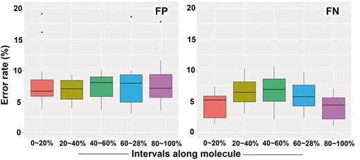
Distribution of false-positive (FP) and false-negative (FN) signals along whole molecules. BioNano molecules are divided into five equal-sized intervals, 0–20, 20–40, 40–60, 60–80 and 80–100%. For FN rates, pairwise comparison between three middle interval groups (20–40, 40–60, 60–80%) and two outside groups (0–20, 80–100%) showed the three middle interval groups significantly differed from the two outside groups (t-test: P < 0.05)

3.1.3 Data variations due to the stretching of DNA molecules

Stretching of DNA molecules under various conditions, e.g. salt concentration, temperature, electrical field strength, nano-channel pore size, etc. may cause changes in the measured length of BioNano molecules, thus affecting downstream applications such as mapping or the assembly of BioNano molecules. We investigated the changes in the stretch variation factor (Section 2) between nanochips, between flow cells of the same chips, between runs for the same flow cells, and between scans within a run.

First, although no difference in the stretch variation factor was detected between flow cells within the same nanochips (Supplementary Fig. S3, second row, Chip2 Flowcell1 versus Chip2 Flowcell2: Kruskal-Wallis rank-sum test, P > 0.05), a significant difference in the stretch variation factor was observed between different nanochips (Supplementary Fig. S3, first row, Chip1 versus Chip2; Kruskal-Wallis rank-sum test, P < 0.05). Second, in practice, multiple runs (with the same sample preparation) were often applied to the same flow cells, for which a new run was often started with the addition of a new sample volume. Changes in the stretch variation factor between different runs of the same flow cells can occasionally be significant (Supplementary Fig. S3, third row; and Supplementary Fig. S4G). Changes in the stretch variation factor between different runs were found to be larger than within the same run. Third, considering the scans within runs, we found that the stretch variation factor decreased during a single run (Supplementary Fig. S3, fourth row). Reduction in stretch variation factor were the result of the increased salt concentration (Kim et al., 2011). We noticed that higher flow rates and a short run time reduced the impact of salt concentration on the stretching variation (Supplementary Fig. S4F). We further considered the distribution of the stretch variation factor for molecules of the same run. They were found to approximate a Gaussian distribution (Supplementary Fig. S5; Section 2.4), which was used to model the DNA molecule stretch variation in the BioNano molecule simulator BMSIM.

3.1.4 Variation in the optical resolution of the BioNano system and its modelling

We investigated the resolution within our BioNano datasets that was likely a combined function of many variables. By aligning BioNano molecules to their reference sequences, we analyzed the distribution of neighbouring labelling sites, and their relationship to distance on the reference genome. We found that neighbouring sites within 1–3 Kb of each other were only partially resolved by BioNano with resolution limit approaching 1 Kb (Fig. 2). The likelihood of two labelling sites being distinguished decreased as the distance between them was reduced from 3 to 1 Kb, which was modelled as a cumulative Gaussian distribution (Section 2.5). The fitness of the model to the observed data was confirmed using a curve fitting test (Fig. 2). Notably, the eight BioNano datasets displayed a high consistency in curve fitting. In addition to the optical resolution that determines the minimum detectable unit, the presence of restriction sites in a region is required to map structural features by BioNano. Thus, the frequency of restriction sites is another important factor limiting the detectability of the BioNano genome mapping system. Based on the profile, the variation in optical resolution for BioNano molecules was modelled as a cumulative Gaussian distribution in the BioNano molecule simulator BMSIM (Section 2.5).

Fig. 2.

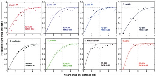
Variation in the optical resolution of the BioNano system, as revealed by the ratio distribution of resolved neighbouring sites in BioNano molecules from eight organisms. ‘Resolved neighbouring site ratio’ represents the ratio of the resolved neighbouring sites to the total neighbouring sites on BioNano molecules at the same distance. Dots are the distribution for BioNano molecule data, and lines represent the fitting curves of the cumulative Gaussian distribution. R2 (coefficient of determination) and RMSE (root mean squared error) were computed for each dataset

3.1.5 Formation of chimeric molecules

The formation of chimeric molecules from the joining of multiple unrelated genomic regions has not been systematically characterized for the BioNano genome mapping system to date. Because the BioNano experiments did not involve PCR or DNA-ligation steps, the chimerism most likely resulted from the concatenation of random DNA molecules in nanochannels during imaging. By analyzing the BioNano molecules that were aligned to two or more regions in the reference genome, we identified the joining of two, three or more BioNano molecules from unrelated genomic regions (Fig. 3A). Among the eight BioNano datasets, on average, ∼15% of all molecules were chimeric (Fig. 3B and C) and shared a similar profile of chimerism. ‘Bimera’ was the most common type, accounting for ∼87% of all chimeric instances. Higher-order chimeras, such as ‘Trimera’ and ‘Quadramera’, occurred at a much lower frequency, accounting for ∼12 and ∼1%, respectively. Considering the frequency of chimeric events for molecules of different length, not surprisingly, we found that longer molecules generally had a higher frequency of chimeric events (Fig. 3D). For example, molecules longer than 300 Kb were found to have an approximately 30% chance to be chimeric.

Fig. 3.

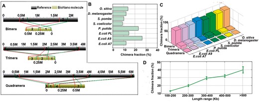
Formation of chimeric BioNano molecules. (A) Examples of chimeric molecules identified in our E.coli sample sets. To identify a chimaera, some more stringent thresholds were used, i.e. mapping confidence score >8 (for anchoring molecule regions to reference genome) and the ratio of the anchored regions to the total molecule length >70%. The lines represent the boundary for aligned regions between chimeric molecules and reference genomes. (B) Chimera fraction detected for each BioNano molecule dataset. (C) Proportion of Bimera, Trimera and Quadramera among all chimeric molecules for each BioNano molecule dataset. (D) Longer molecules having a higher rate of chimeric events

3.1.6 Coverage distribution bias and fragile sites

BioNano molecules should distribute uniformly over genomes because of the shotgun process. Ignoring the edge effect, it was an equivalent of a homogeneous Poisson process (Sarkar, 2006). To examine the coverage uniformity, we aligned the BioNano molecule data to those of reference genomes and tabulated the coverage depth per labelling site for each genome to produce coverage density plots (Fig. 4A). The coverage distributions of P.pudita and D.melanogaster were found to deviate from theoretical Poisson distribution. To identify the cause of deviation, we looked more closely at the P.Putida dataset, which had over 1000-fold average coverage and severe deviation (Fig. 4A). Eight spots with dramatically lower coverage were found to correspond to so-called fragile sites in the P.putida genome (Fig. 4B, dots).

Fig. 4.

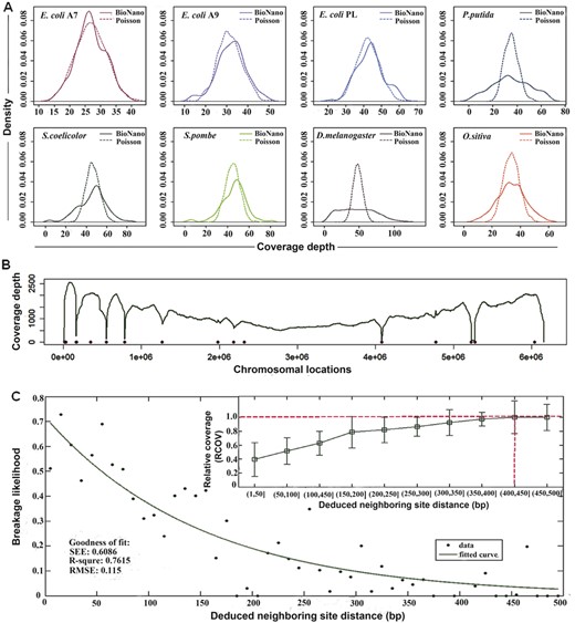
Coverage distribution bias and fragile sites of BioNano molecules. (A) Density plots of the coverage depth per labelling site for eight organisms. The solid (BioNano) and dashed (Poisson) lines represent the distributions of real molecules and the theoretical Poisson model with the same mean, respectively. Note that the gap regions and mapped outliers (count greater than two times the median count) along the chromosome are excluded. (B) Coverage depth and fragile sites along the P.putida genome. The dots represent the predicted fragile sites. (C) Curve fitting of the breakage likelihood versus deduced neighbouring site distance. The distance between two neighbouring sites was deduced based on their locations on the reference genome. The breakage likelihood of fragile sites is designated 1 minus the relative coverage (RCOV) at potential fragile sites. The relative coverage (RCOV) is the ratio of the coverage depth at a fragile site to the average coverage depth of the whole genome. The inner panel illustrates the distribution of RCOV versus the binned neighbouring sites distance. When the distance between neighbouring sites increases to ≥400 bp, RCOV is close to 1, indicating a low (near 0) likelihood of breakage. SSE, the sum of squares due to error; R-square, coefficient of determination; Adjusted R-square, degree-of-freedom adjusted coefficient of determination; RMSE, root mean squared error

To determine the distance range between sites in a fragile site, we plotted the likelihood of breakage against the distance between nicking sites on opposite strands (Fig. 4C inner panel). The likelihood of breakage was estimated using the relative coverage of aligned molecules, i.e. a lower coverage representing higher breakage likelihood. We concluded that a fragile site was likely to form when two nicking sites on opposite strands were within 400 bp of each other (Fig. 4C inner panel, dash line). The potential fragile sites for the eight datasets in our study were calculated (Supplementary Table S2). The likelihood of breakage increased as the two nicking sites on opposite strands getting closer to each other, following a curve approximating exponential decay (R² = 0.7615; Fig. 4C) (Section 2.6).

Uneven labelling density along a genome was another factor that might contribute to coverage bias. By analyzing the relationship between the uniformity of the labelling site distribution and coverage depth, we found a correlation (averaged R = 0.41) between the local label density (labelling sites/100 Kb) and the relative coverage depth, indicating a biased coverage against genome regions with sparse labelling sites. The existence of large sparse labelling regions in the P.pudita genome (R = 0.63), and D.melanogaster genome (R = 0.76), may explain their derivations from theoretical Poisson distribution in coverage depth. Apart from fragile sites and uneven labelling site distribution, molecule length, alignment parameters (Supplementary Figs S6 and S10) as well as repetitive elements, gaps and ambiguous sequences in reference genomes, DNA stretching variations, FN or FP errors and chimeric molecules may play a role in making coverage distribution over-dispersed and/or skewed.

3.2 BioNano molecule simulator (BMSIM)

Based on the properties and statistical models of the BioNano molecule data (detail information of the models can be found in Section 2 and Supplementary Methods), we developed a program, BioNano Molecule SIMulator (BMSIM), to generate BioNano molecules data in silico. BMSIM comprises five major steps: in silico fragmentation, nicking site labelling, error modelling, SNR score assigning and coverage depth iteration (Fig. 5). To evaluate the performance of BMSIM, we generated simulated BioNano molecule data for four organisms (E.coli PL, P.putida, S.pombe and O.sativa). The synthetic datasets were found to closely match the measured properties of the experimental data (Supplementary Table S3). Remarkably, BMSIM reproduced coverage bias due to fragile sites. When the function for simulating fragile sites was disabled for BMSIM, the signature of fragile site bias, i.e. reduced coverage depth at fragile sites disappeared (Supplementary Fig. S7).

Fig. 5.

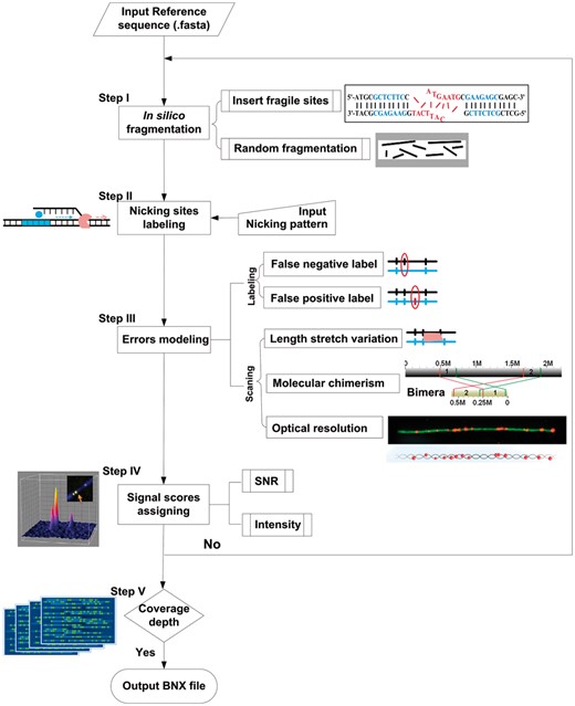
Scheme diagram of BioNano Molecule SIMulator (BMSIM). BMSIM comprises of five major steps: in silico fragmentation, nicking sites labelling, error modelling, SNR score assigning and coverage depth iteration (see Supplementary Methods Section S1.3 for details)

3.3 Evaluation of factors impacting whole-genome optical map assembly using simulated BioNano data

The assembly of a whole-genome optical map is an essential application of BioNano genome mapping technology, which can facilitate the construction of a reference genome, resolving highly repetitive sequences and correcting of some gnome assembly errors. The factors that impact whole-genome optical map assembly have not been systematically investigated, and their effects have not been quantitatively evaluated. Thus, it is imperative to investigate how whole-genome optical map assembly is affected by the biases and errors of BioNano molecule data and to seek the optimal conditions/parameters under which the best practice of BioNano experiments should be carried out.

To perform the study, we used synthetic datasets generated with BMSIM, which simulated broad data features/conditions that were not possible without the BioNano data simulator. The simulated datasets were assembled using the BioNano in-house Assembler Version 3370 from the IryView package. The analysis was designed to investigate the effects that factors such as coverage depth, molecule length, FN/FP errors, chimerism, enzyme selection and nicking/labelling site density had on the outcome of whole-genome optical map assembly.

3.3.1 Coverage depth of BioNano molecule data

Coverage depth is a critical factor for the design of BioNano experiments. To estimate the sensitivity and specificity at various coverage depths, we generated simulated BioNano data for four organisms of various genome sizes: S.coelicolor, H.sapiens, D.melanogaster and O.sativa. Although the other factors, e.g. average length, FN/FP, nicking site density and chimeric molecules, remained constant among the four datasets, each genome was assembled with BioNano molecule data of various coverage depths between 10× and 100× (Fig. 6A). The results of assemblies were evaluated with assembly completeness, contig N50 and contig number. While a high assembly completeness (95%) was achieved at 40× coverage depth for a smaller genome, larger genomes required a much higher coverage depth (100×) to reach the same level. However, contig N50 behaved similarly among the genomes below 80× coverage depth and started to differentiate above that point (Fig. 6A middle panel). Notably, for large genomes, e.g. D.melanogaster and O.sativa, a coverage depth of 80× was required to have a contig N50 larger than 1 Mb. For assembly fragmentation, we observed that the number of contigs increased initially before it was reduced (Fig. 6A right panel). The turning point was intrinsic to each genome, probably closely related to its genome size.

Fig. 6.

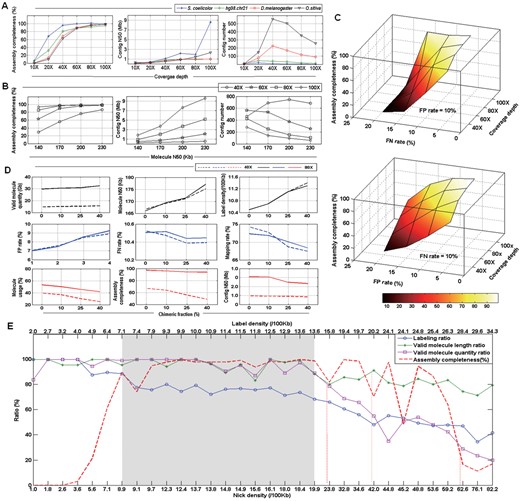
Simulation study of whole-genome optical map assembly using synthetic BioNano molecule data by BMSIM. (A) Effect of coverage depth on results of whole-genome optical map assembly. Assembly completeness is the ratio of assembled map size to reference genome size. (B) Effect of BioNano molecule length (N50) on results of whole-genome optical map assembly. The genome of O.sativa, IRGSP1.0, was used in the simulation analysis. (C) Impact of FP/FN error rates on results of whole-genome optical map assembly. The genome of O.sativa, IRGSP1.0, was used in the simulation analysis. The variable error rate of 0.05, 0.10, 0.15 and 0.20 was simulated with the other one fixed at 0.1, and coverage depth at 40, 60, 80 and 100×. The result plane of variable FN rates has a steeper slope than that of variable FP rates. (D) Effect of different chimera fractions on results of whole-genome optical map assembly. The genome of O.sativa, IRGSP1.0, was used in the simulation analysis. (E) Effect of nicking enzyme selection and nick site density on results of whole-genome optical map assembly. Synthetic BioNano molecule data were generated in silico with sampled genomes of the eight organisms with different GC contents (Supplementary Table S4) using four nicking enzyme, Nt.BspQI, Nb.BbvCI, Nb.Bsml and Nb.BsrDI. Labelling ratio, the ratio of labelling density to nick density; valid molecule length ratio, the ratio of valid molecule (>100 Kb) N50 with fragile sites to valid molecule (>100 Kb) N50 without fragile sites; valid molecule quantity ratio, the ratio of valid molecule (>100 Kb) quantity with fragile sites to valid molecule quantity (>100 Kb) without fragile sites; assembly completeness, the ratio of assembled map size to reference genome size

3.3.2 Molecule length of BioNano molecule data

The length of BioNano molecules can vary greatly depending on the organism, experimental protocol for DNA isolation, and often the skill of the researcher. Thus, we determined whether the length of the BioNano molecules (assuming the same standard distribution as described above) impacts the outcome of map assembly. We generated synthetic BioNano molecule data of the O.sativa genome (∼380 Mb), with N50 lengths at 140, 170, 200 and 230 Kb and coverage depths fixed at 40, 60, 80 and 100×. Our results showed that, at a lower coverage depth, the molecule length had a greater impact on the assembly completeness (Fig. 6B, left panel). However, a larger molecule length needed only a low coverage depth to achieve a high completeness rate. As the molecule length increased, contig N50 became larger, accompanied by the decrease in the contig number (Fig. 6B middle and right panels).

3.3.3 FP/FN errors of BioNano molecule data

The FN and FP rates of the BioNano data varied depending on the quality of DNA samples and conditions of the nicking/labelling reactions. It was unclear how FN and FP errors impacted the outcome of whole-genome optical map assembly. Using BMSIM, we generated simulated BioNano data for O.sativa (∼380 Mb) with combinations of different FN and FP rates (5, 10, 15 and 20%). For this analysis, the coverage depth was fixed at 40, 60, 80 and 100×.

The result plane of variable FN rates had a steeper slope than that of variable FP rates (Fig. 6C), suggesting the FN rate had a greater influence on whole-genome optical map assembly completeness than the FP rate. The assembly completeness dropped sharply from 99 to 0.04, 0.07, 0.5 and 2% as the FN rate increased from 5 to 20% for the coverage depths of 40, 60, 80 and 100×, respectively (Fig. 6C). On the other hand, the assembly completeness decreased from 99 to 7, 20, 36 and 49% as the FP rate increased to the same extent. However, at high error rates, e.g. 20%, of either FP or FN, the result of whole-genome optical map assembly became unacceptable. An increased coverage depth may have been able to compensate for the slightly elevated error rates of FP or FN. For example, with an FN rate of 15% (FP = 10%), the coverage depths of 80× and 100× led to assembly completeness values of 50 and 95%, respectively (Fig. 6C). With an FP rate of 15% (FN = 10%), the coverage depths of 80× and 100× resulted in assembly completeness values of 67 and 81%, respectively.

3.3.4 Chimerism of BioNano molecule data

Molecule chimerism is a common issue for BioNano molecule data and might cause assembly errors using overlapping graphs. To evaluate the impact of chimeric molecules on whole-genome optical map assembly, simulated BioNano molecule data (with coverage depths of 40× and 80×) were generated for O.sativa with chimera fractions at 0, 10, 25 and 40%. Whereas chimeric molecule artificially increased the valid molecule quantity (>100 kb), the molecule length, label density, FP rate and FN rate changed little (Fig. 6D). In contrast, as the chimera fraction increased, the molecule mapping rate, the molecule usage, the assembly completeness and contig N50 were reduced. Further, the assembly with lower coverage molecule data had a much greater impact in the presence of chimeric molecules (Fig. 6D). Notably, the experimentally generated BioNano datasets had an average chimera fraction between 8.7 and 26.4% (Fig. 3B). Thus, molecule chimerism is an important factor when considering BioNano experiments for whole-genome optical map assembly. To minimize the chimeric rate, we may reduce the DNA concentration when running DNA samples through nanochips.

3.3.5 Choice of nicking enzyme and nick site density

The choice of nicking enzyme is genome specific and critical to produce informative data for whole-genome optical map assembly. BioNano currently offers the choice of four nicking enzymes for labelling, Nt.BspQI, Nb.BbvCI, Nb.Bsml and Nb.BsrDI. To understand how different enzymes and their nicking patterns affect the outcome of whole-genome optical map assembly, we designed and performed a comprehensive analysis using sample genomes of organisms with different GC content, D.discoideum (GC% = 23), S.ratti (GC% = 22), A.thaliana (GC% = 37), H.sapiens (GC% = 41), D.melanogaster (GC% = 43), O.sativa (GC% = 44), P.putida (GC% = 63) and S.coelicolor (GC% = 73) (Supplementary Table S4). BioNano molecule data were generated in silico with the four available nick enzymes using BMSIM, producing a spectrum of nick site densities ranging from 1.0 to 82.2/100 Kb that were translated to labelling densities ranging from 2.0 to 34.3/100 Kb due to the collapse of nearby sites (Fig. 6E, and Supplementary Table S4).

The properties and quality of simulated BioNano molecule data were evaluated using the labelling ratio (ratio of the labelling density to the nicking density), valid molecule (>100 Kb) length ratio (ratio of the valid molecule length with fragile sites to that without fragile sites) and valid molecule (>100 Kb) quantity ratio (ratio of the valid molecule quantity with fragile sites to that without fragile sites). As expected, assuming an optimized nicking reaction protocol, we observed a decrease in the labelling ratio, valid molecule length ratio and valid molecule quantity ratio with the increase in nick site density (Fig. 6E) because a higher nick density would result in more fragile sites, thus making the molecule length shorter. For example, with a nick site density at 23.85/100 Kb, the labelling density was 15.8/100 Kb, a ∼34% drop in the labelling ratio, a ∼20% drop in the valid molecule length ratio and a ∼22% drop in the valid molecule quantity ratio. In the extreme case of a nick site density at 62.6/100 Kb, the labelling density would be 28.4/100 Kb, with a 70% decrease in the valid molecule quantity ratio. Thus, for enzymes that produced a high nick site density, the reduction of the labelling ratio and valid molecule became significant.

Next, we evaluated the effects of nicking enzymes and the nicking site density on the outcome of map assembly. We observed that although the labelling density ratio remained high at low nick site density (<8.9/100 Kb; labelling density < 7.1/100 Kb), the assembly completeness was poor (Fig. 6E, dash line). In contrast, at a high nick site density (>42.0/100 Kb; labelling density > 20.2/100 Kb), a 50% drop in the labelling density led to the assembly completeness dropping significantly to below 80%. Thus, decreasing the labelling ratio is an important signal to monitor, and new experiments may be warranted if the ratio becomes too low.

Considering the results, it was suggested that enzymes with a nick site density above 40/100 Kb or below 9.0/100 Kb should be avoided. For enzymes with a nick site density in the range of 20–40/100 Kb, the labelling ratio, valid molecule length ratio, valid molecule quantity ratio and assembly completeness declined substantially. Hence, a nick site density between 9 and 20/100 Kb (labelling site density between 7 and 14/100 Kb) would be optimal to guarantee high-quality molecule data and complete map assembly at an acceptable cost (Fig. 6E, shaded regions).

4 Discussion

To investigate the property, bias and error profile of BioNano data, we generated BioNano molecule data and exploited organisms with varying genome sizes. Although we revealed many common descriptive properties for physical mapping data, some pertain only to the BioNano system. Summary of the properties of BioNano data and the observation of these properties are listed in Supplementary Table S6. The FP and FN signals are distributed differently for BioNano molecules. While FP signals are random events with a physically uniform distribution along DNA molecules, FN signals are elevated in the middle intervals of DNA molecules, attributed to the tertiary structure of DNA molecules in nicking and labelling reaction solutions that limit the access of enzymes. DNA molecule stretching varies between different nanochips, runs and scans and is likely affected by factors such as nano-channel size, labelling reagent and salt concentration. Optical resolution of the BioNano system varied with the low boundary approaching ∼1 Kb, whereas neighboring sites within 1 Kb of each other may be detected but un-reliable. The likelihood of two neighbouring sites within 1–3 Kb being resolved follows a cumulative Gaussian distribution. Chimeric molecules, on average, account for ∼15% of total molecules and have a substantially higher frequency for longer DNA molecules (>300 Kb). A good option is to reduce chimeric rates of long molecules, by removing long molecules with a backbone intensity greater than a certain threshold that are likely chimeric. Additional work is needed to explore the method to detect the cases of multi-molecule pileups in nano-channel, and exam its relationship with occupancy. The coverage distribution of BioNano molecules is found to be deviated from homogeneous Poisson, for which fragile sites, sparse labelling, molecule length, repetitive elements, DNA molecule stretching variation, chimerism and reference genome quality, among others, are likely contributing factors. For whole-genome optical map assembly, low coverage due to sparse labelling can be remedied by increasing the overall molecule length or total BioNano data. However, higher coverage depth is often useless for fragile sites. For example, although up to 1783× BioNano molecule data were generated for P.putida, its whole-genome optical map assembly was still fragmented due to break-up at four fragile sites. For such cases, we propose that a ‘stitching’ procedure utilizing rare molecules covering fragile sites or a combination of BioNano maps with different nicking enzymes can be explored. In addition, algorithmic enhancements to BioNano pipeline, for example, normalization for DNA molecule stretching, chimeric molecule analysis with split/partial alignments or detection/filtering of false signals, may be pursued to improve optical data mapping and genome map assembly.

Coverage depth and molecule length are two essential variables for BioNano experiments, and it is important to put them in perspective for whole-genome optical map assembly. It is apparent that as genomes become larger, coverage depth becomes more critical for the three measurements of whole-genome optical map assembly: the assembly completeness, contig N50 and contig number (Fig. 6A). Under normal experimental conditions, a 40× to 60× coverage depth is sufficient for the map assembly of bacterial genomes, but an 80× to 100× coverage depth is required for eukaryotic genomes over 100 Mb in size. When the assembly completeness approaches 100%, the contig N50 and contig number for whole-genome optical map assembly continue to improve with higher coverage. Thus, we recommend even higher coverage when designing BioNano experiments for applications that desire long continuity of whole-genome optical maps. Increasing the length of BioNano molecule data has a significant effect (somewhat surprising) on the quality of whole-genome optical map assembly, as evidenced by the near linear correlation between molecule length and completeness of assembly, contig N50 and contig number (Fig. 6B). Although these results demonstrate the benefit of a large molecule length in whole-genome optical map assembly, more often in practice, the benefit of a large molecule length is not achievable due to the technical difficulty to preserve long DNA through isolation and labelling steps.

FP/FN signals and chimeric molecules are two intrinsic factors that may not be easy to control or manipulate. However, it is critically important to understand the impact of their variations on whole-genome optical map assembly. FP/FN signals are found to have an uneven effect on whole-genome optical map assembly, with an increase in the FN rate having a greater influence than that in the FP rate (Fig. 6C). We suggest using a sufficient amount of enzyme and possibly a longer reaction time in the nicking/labelling steps to keep the FN rate low. Additionally, based on simulation results, the quality filter parameter ‘snrFilter’ in BioNano assembly pipeline can be relaxed to avoid missing true positive signals with the cost of a slightly higher FP rate. Furthermore, an increased coverage depth may be recommended to mitigate the effect of elevated FN and FP rates for whole-genome optical map assembly. Note that, among the eight BioNano datasets generated experimentally, the FP and FN rates were found to be no greater than 9.04 and 15.9%, respectively (Supplementary Table S1). Thus, for genomes over 100 Mb in size, a coverage depth of 80× to 100× should be at least considered for whole-genome optical map assembly. The effect of chimeric molecules on whole-genome optical map assembly was found to be more severe at a low coverage depth than at high coverage ones (Fig. 6D). However, at a higher coverage depth (e.g. ≥80×) the impact of chimeric molecules on whole-genome optical map assembly was minimized.

Nicking enzyme selection is often the first decision to make in BioNano experiments. Researchers often rely on general suggestions from BioNano to perform test runs for an unknown genome. By simulating the whole spectrum of nicking and labelling densities with combinations of enzymes and synthetic datasets of organisms with variable GC content, we revealed a complete picture of variable nicking/labelling densities with the outcome of whole-genome optical map assembly. With higher nicking densities, increases in fragile sites and FN rates severely reduce the labelling ratio, valid molecule length ratio and valid molecule quantity ratio. In particular, the decrease in the labelling ratio is the benchmark signal to monitor. With the labelling ratio decreasing to 50%, whole-genome optical map assembly collapses and becomes unacceptable in terms of completeness and fragmentation. In such a scenario, new experiments with different nicking enzymes should be pursued. Our results demonstrate that a nick site density between 9 and 20/100 Kb (labelling site density between 7.0 and 14/100 Kb) is the optimal range for BioNano experiments. For a new organism, these parameters may be estimated using a closely related genome or Illumina sequencing data. Further, to develop a guideline on how to choose appropriate nicking enzymes for organisms of various GC contents, we obtained a total of 128 genomes covering broad phylogenetic systems (Supplementary Table S7). Basing on their nicking/labelling density predicted using recognition sequences of nicking enzymes, we recommend the nicking enzymes Nb.Bsml and NbBsrDl for genomes with a low GC content (<25%), Nt.BspQI for those with a medium GC content (25–40%), and both Nt.BspQI and Nb.BbvCI for those with a higher GC content (>40%) (Supplementary Fig. S11). BMSIM simulator can be extended to other applications. For example, it can help investigate on the robustness of haplotype-sensitive assembly for various BioNano data. By simulating haplotype blocks of various length for diploid genomes, the accuracy and sensitivity of haplotype-sensitive assembly can be evaluated.

Funding

This work was supported in part by grants from the Ministry of Agriculture of China (2016ZX08010-002), the National Science and Technology Major Projects (2018ZX09711003) and the National Natural Science Foundation of China (Nos. 31401128, 31571310, 31771412) and by Special Fund for Strategic Pilot Technology Chinese Academy of Sciences (XDA08020104).

Conflict of Interest: none declared.