Robust clustering of noisy high-dimensional gene expression data for patients subtyping

Abstract

Motivation

One of the most important research areas in personalized medicine is the discovery of disease sub-types with relevance in clinical applications. This is usually accomplished by exploring gene expression data with unsupervised clustering methodologies. Then, with the advent of multiple omics technologies, data integration methodologies have been further developed to obtain better performances in patient separability. However, these methods do not guarantee the survival separability of the patients in different clusters.

Results

We propose a new methodology that first computes a robust and sparse correlation matrix of the genes, then decomposes it and projects the patient data onto the first m spectral components of the correlation matrix. After that, a robust and adaptive to noise clustering algorithm is applied. The clustering is set up to optimize the separation between survival curves estimated cluster-wise. The method is able to identify clusters that have different omics signatures and also statistically significant differences in survival time. The proposed methodology is tested on five cancer datasets downloaded from The Cancer Genome Atlas repository. The proposed method is compared with the Similarity Network Fusion (SNF) approach, and model based clustering based on Student’s t-distribution (TMIX). Our method obtains a better performance in terms of survival separability, even if it uses a single gene expression view compared to the multi-view approach of the SNF method. Finally, a pathway based analysis is accomplished to highlight the biological processes that differentiate the obtained patient groups.

Availability and implementation

Our R source code is available online at https://github.com/angy89/RobustClusteringPatientSubtyping

Supplementary information

Supplementary data are available at Bioinformatics online.

1 Introduction

Many diseases—for example, cancer, neuro-psychiatric and autoimmune disorders—are difficult to treat because of the remarkable degree of variation among affected individuals (Saria and Goldenberg, 2015). Precision medicine (Hood and Friend, 2011) tries to solve this problem by individualizing the practice of medicine. It considers individual variability in genes, lifestyle and environment with the goal of predicting disease progression and transitions between disease stages, and targeting the most appropriate medical treatments (Mirnezami et al., 2012).

A central role in precision medicine is played by patient sub-typing, that is the task of identifying sub-populations of similar patients that can lead to more accurate diagnostic and treatment strategies. Identifying disease sub-types can help not only the scientific areas of medicine, but also the practice. In fact, from a clinical point of view, refining the prognosis for similar individuals can reduce the uncertainty in the expected outcome of a treatment on each individual.

Being able to accurately estimate the outcome (survival) of the disease is the key in the successful treatment of cancer patients. This estimation depends on clinical or laboratory factors that are linked to patient outcomes.

The most common approach used in the outcome estimation of cancer patients is based on composite index categorization, that assign patients to different stage levels based on clinical variables that depend on the type of disease. One example is the TNM index (Tumor, Lymph Nodes and Metastasis) that was defined to classify the progression of cancer that originates from solid tumour. Thus, the outcome estimation is based on the survival estimation of the patients in each stage (Green et al., 2006).

Then, with the advent of high-throughput omics-technologies, using statistical and machine learning approaches such as non-negative matrix factorization, hierarchical clustering and probabilistic latent factor analysis (Brunet et al., 2004; Perou et al., 2000), researchers have identified subgroups of individuals based on similar gene expression levels. Moreover, several data integration approaches for patient subgroup discovery were recently proposed, based on supervised classification, unsupervised clustering or bi-clustering (Planey and Gevaert, 2016; Higdon et al., 2015; Liu et al., 2016; Taskesen et al., 2016) To improve the model accuracy for patient stratification, other omics data types can be used, such as miRNA (microRNA) expression, methylation or copy number alterations, in addition to gene expression. For example, somatic copy number alterations provide good biomarkers for cancer subtype classification (Vang Nielsen et al., 2008). Data integration approaches to efficiently identify sub-types among existing samples have recently gained attention. The main idea is to identify groups of samples that share relevant molecular characteristics.

All these methods strongly depend on the similarity measure used in the analysis and are sensible to the noise in the experimental data. Moreover, these methodologies, do not guarantee a good separability of the patients in terms of survival.

Recently, a fully Bayesian approach (called SBC), able to cope with the last problem, was proposed (Ahmad and Fröhlich, 2017). The SBC method performs the clustering analysis by jointly analysing omics and survival data. It is a semi supervised method, since it uses a lasso based Accelerated Failure Time (AFT) model to identify the feature that better correlate with patient survival times. Then a Hierarchical Bayesian Graphical Model is applied to combine a Dirichlet Process Gaussian Mixture Model with the AFT model to identify the clusters that have a good separability in terms of omics signatures and survival time, and being able to predict the survival time for new patients.

In this study, we propose a new computational framework that, unlike SBC, is able to solve the two aforementioned problems in an unsupervised manner. Indeed, it aims to combine robust and sparse gene correlation estimation, an unsupervised clustering algorithm robust to noise and survival analysis, in order to find patient subtypes that have also a good survival separability. The methodology is described in Figure 1.

Fig. 1.

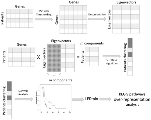
The proposed approach for clustering patients is composed of several steps. First of all, starting from the gene expression data matrix, the robust and sparse gene co-expression matrix is computed with the RSC method. RSC also identifies the optimal threshold to cut spurious correlations. Then, the correlation matrix is decomposed into its spectral components (eigenvalues and eigenvectors). Only the first m components of the decomposition are used to project the patients onto a rotated subspace. In this subspace, the OTRIMLE algorithm is applied. Survival curves were computed for the obtained clustering. Separation of survival curves is evaluated for each clustering solution. The (optimal) clustering that maximizes survival curves separation is chosen. Based on the optimal clustering, the differentially expressed genes are computed (starting from the original matrix) for each cluster versus the others. Finally, to give more insights into the biological process underlying the patients cluster, a pathway over-representation analysis is performed

The proposed methodology, described in the beginning of Section 2, is a combination of robust dimensional reduction techniques and clustering. In a nutshell: a cluster solution on a data subspace is searched that has good properties in terms of survival curves separation. The method looks for many candidate clustering solutions, and chooses one that is optimal according the survival empirical evidence. The proposed method handles noise and outliers, very common in this kind of data, in a fully adaptive and unsupervised way. It is cheaper, in terms of data acquisition, than modern multi-view methods and performs remarkably competitive on five datasets. In fact, we tested our methods on five real cancer datasets downloaded from the TCGA website, and we compared our survival curve separation with that obtained by using the similarity network fusion (SNF) algorithm, and model based clustering based on Student’s t-distribution (TMIX) of Peel and McLachlan (2000) on the same data. Our experiments suggest that our method outperforms the SNF and TMIX methods in terms of survival curves separability. On the other side, since OTRIMLE is a combination of robust methodologies, it is computational more expensive than SNF and TMIX.

The rest of the article is organized as follows: first we explain our methodology, discussing about the needing of a robust correlation estimator and of a clustering method robust to noise. Then we present a new measure to compute the distances between survival curves. Finally, experimental results are presented.

2 Materials and methods

Suppose we have a set of p genes measured on n samples, data are stored in the $n\times p$ data matrix $\mathbf{X}={\left[x_{l,m}\right]}_{l=1,2,\dots ,n}^{m=1,2,\dots ,p}$⁠. Measurements on the ith unit (patient) are given by ${\mathit{x}}_i={(x_{i,1},x_{i,2},\dots ,x_{i,p})}^{\prime }$⁠, while the lth column (that is the lth gene) is denoted by $X_l=(x_{1,l},x_{2,l},\dots ,x_{n,l})$⁠. We want to discover k clusters within the patients (rows of $\mathbf{X})$⁠. The proposed methodology for the analysis of gene expression data for patient subtyping consists of the following steps:

• 1. build the gene co-expression matrix by using the Robust and Sparse Correlation matrix estimator (RSC) of Serra et al. (2017). Perform the spectral decomposition of the RSC matrix so that the eigenvalues are in non-increasing order.

• 2. Fix an integer m > 1, and a real number $\gamma \ge 1$⁠, and do the following:

•    a. project the rows of the original gene expression matrix X onto the space spanned by the first m eigenvectors of the RSC matrix obtaining a $\mathbf{Z}\left(m\right)$ matrix of dimension $(n\times m)$⁠;

•   b. perform the OTRIMLE clustering method of Coretto and Hennig (2016) and Coretto and Hennig (2017) on the rows of $\mathbf{Z}\left(m\right)$⁠. This requires the regularization parameter γ called the ‘eigenratio constraint’ (explained in details in Section 2.2);

•   c. estimate the survival curves cluster-wise based on non-parametric methods, and evaluate the separation between the k clusters in terms of survival curve separation.

Steps 2(a)2(c) are performed for several combinations of values for m and γ obtaining a number of cluster solutions.

• 3. The final clustering is chosen so to maximize the separation in terms of survival curves given that the associated P-value is satisfactory.

• 4. For each cluster, a list of over-represented pathways are identified that distinguish that cluster from the others.

In the following sections each step of the analysis is disentangled.

2.1 Data projection based on the RSC estimator

One of the major issues in clustering analysis is the high-dimensionality of the feature space, that is the number p of genes. In high dimension, the feature space becomes geometrically sparse and most of the clustering methods are prone to degrade their performance. The ideal would be to reduce the data dimension by filtering out those genes that do not contribute to the clustering, but this is not generally known. A traditional approach is to project the original data matrix onto a space of lower dimension m < p. The most popular of such methods is the Principal Component Analysis (PCA), that is the data matrix is projected onto a lower-dimensional space spanned by a subset of m < p eigenvectors of the sample covariance or correlation matrix to which are associated the corresponding m largest eigenvalues. Unfortunately, the typically small concentration ratio p/n drives the bias of the estimated spectral components to huge levels affecting the final analysis. Moreover, it is well-known that gene arrays are rich of outlying measurements (see Marshall, 2004), and only a few of them can completely breakdown the sample covariance/correlation matrix. In Serra et al. (2017) these issues are treated in detail. The Robust and Sparse Correlation matrix estimator (RSC) proposed in Serra et al. (2017) was shown to successfully jointly tame both the effects of a small concentration ratio, and the influence of outlying measurements. Robustness is achieved by replacing the sample correlation matrix with an ensemble of robust pairwise correlation coefficients due to Pasman and Shevlyakov (1987). Sparsity of the resulting correlation matrix is obtained based on an adaptive thresholding method. The RSC estimator is simple to compute, and it is completely unsupervised because it does not require data dependent tunings. Let R be the RSC estimate. R is a ‘cleaned’ estimate of the joint correlation structure acting on the measured data. In analogy with PCA, we consider its spectral components. Let ${\lambda }_1\ge {\lambda }_2,\dots ,\ge {\lambda }_p$ be eigenvalues of RSC rearranged in non-increasing order, and let $\mathbf{\Lambda }=\text{diag}({\lambda }_1,{\lambda }_2,\dots ,{\lambda }_p)$ the diagonal matrix containing them. Let $\mathbf{\Gamma }$ be the matrix whose columns are normalized eigenvectors associated to $({\lambda }_1,{\lambda }_2,\dots ,{\lambda }_p)$⁠. Therefore, $\mathrm{R}=\mathbf{\Gamma }\Lambda {\mathbf{\Gamma }}^{\prime }$⁠. Column vectors of $\mathbf{\Gamma }$ point toward directions of increasing variability as one moves the column index from 1 to p. Let ${\displaystyle \dot{\mathbf{X}}}$ be the centered-scaled data matrix, where each column of the original data is centered onto its median, and scaled according to its median absolute deviation (these are robust alternatives to the sample mean and standard deviation). Let $\mathbf{\Gamma }\left(m\right)$ be the $(p\times m)$ matrix made up of the first m columns of $\mathbf{\Gamma }$⁠, we project the original gene expression data matrix X onto the lower dimensional space spanned by the first m eigenvectors of RSC obtaining $\mathbf{Z}\left(m\right)=\dot{\mathbf{X}}\mathbf{\Gamma }\left(\mathit{m}\right)$⁠. The $(n\times m)$ matrix $\mathbf{Z}\left(m\right)$ is the equivalent of the score matrix in the PCA language. The rows of $\mathbf{Z}\left(m\right)$ represent patients in this reduced and rotated new data space, and these rows are the units to cluster in the following step. In the matrix $\mathbf{Z}\left(m\right)$ a gene is replaced by a linear combination of the expression levels of all genes according to the weight given in the corresponding column of $\mathbf{\Gamma }\left(\mathit{m}\right)$⁠. Therefore, the implicit assumption underlying our analysis is the following: linear combinations of gene expression levels characterize the clustering structure of interest. The eigenvectors of RSC give us a set of candidate interesting directions where to look for such relevant combinations of gene expression levels.

One problem in PCA is the choice of how many orthogonal components to retain in order to preserve most of the observed variance. This corresponds to choose m here. There are good methods for this, however most of these methods are supervised. Moreover, here the main goal of the analysis is different from PCA and similar methods. The problem here is not to explain the total variability contained in X based on a reduced sampling representation $\mathbf{Z}\left(m\right)$⁠. Instead, the aim here is to find a reduced representation of the original data that is able to show valuable clustering information. To this end, m is not chosen based on cumulated variance arguments as in the PCA, but rather we choose an m that is consistent with the cluster separation concept explained in Section 2.3.

2.2 OTRIMLE clustering

Clustering gene expression data is a long-standing problem. Most clustering algorithms are heuristically motivated in absence of theoretical guarantees. The problem of defining what is a ‘good’ clustering solution, is still open. In absence of a well-grounded statistical reference model, it is difficult to answer such questions. These issues are extensively discussed in McLachlan and Peel (2000), Yeung et al. (2001) and McLachlan et al. (2002), where advantages of the model-based clustering approach are shown. One of the major advantages of the model based approach is that assignment is smooth and this allows to better manage situations where one cannot expect a straight separation between the groups. Furthermore, the disastrous effects of even few outlying measurements in clustering analysis are well documented in Hennig (2004) and Escudero et al. (2015). There are few model-based clustering methods that are designed for being outlier/noise-resistant: maximum likelihood (ML) for Gaussian mixtures with uniform noise of Banfield and Raftery (1993), ML for Student’s t-distribution mixtures by Peel and McLachlan (2000), the TCLUST algorithm of García-Escudero et al. (2008) and the OTRIMLE of Coretto and Hennig (2016). Among these, the recently introduced OTRIMLE method has been selected for some of its distinguishing features: (i) the OTRIMLE is fully adaptive to the presence of noise/outliers, and this is essential in multivariate measurements where nobody really knows when noise/outliers are present in the data. (ii) The extensive comparison of Coretto and Hennig (2016) and Coretto and Hennig (2017) showed that OTRIMLE achieves a competitive performance even in extremely adverse noise conditions. It also resulted to be consistent in noiseless situations. (iii) Theoretical guarantees exists [see Coretto and Hennig (2017)] for the robustness of the OTRIMLE method and its algorithm.

The OTRIMLE is now briefly introduced and motivated. It looks for clusters having an elliptical-symmetric shape that can be adequately represented by the contours of the Gaussian density. Assume we want to discover k clusters within n objects on which the feature vector $\mathbf{y}\in {ℝ}^p$ is measured. Let $\{{\mathbf{y}}_i;\hspace{0.17em}i=1,2,\dots ,n\}$ be the sample points. Let $\varphi (\mathbf{y};{\mu }_j,{\mathbf{\Sigma }}_j)$ be the Gaussian density at y centered on the mean vector ${\mu }_j$ with a covariance matrix ${\mathbf{\Sigma }}_j$⁠. The shape of the jth group is described by the level sets of $\varphi (·;{\mu }_j,{\mathbf{\Sigma }}_j)$⁠. Assume that the expected proportion of each group is given by ${\pi }_j\in [0,1]$⁠, with ${\sum }_{j=1}^k{\pi }_j=1-{\pi }_0$⁠, where $0\le {\pi }_0<1$ is the expected proportion of points not consistent with any of the k elliptical-symmetric groups. These points are called ‘noise’, where ‘noise’ means a group of points of arbitrary shape not consistent with the Gaussian prototype. The sampling distribution is represented by the improper mixture density

$${\psi }_{\delta }(\mathbf{y};\theta )={\pi }_0\delta +\sum _{j=1}^k{\pi }_j\varphi (\mathbf{y};{\mu }_j,{\mathbf{\Sigma }}_j),$$

(1)

where δ is the so called ‘noise component’, i.e. a component having positive constant density everywhere in the Euclidean space. Being positive everywhere, the noise component can accommodate even arbitrarily extreme outliers, but it makes $\psi (·)$ an improper density. The parameter vector $\theta$ contains π₀ and all triplets $({\pi }_j,{\mu }_j,{\mathbf{\Sigma }}_j)$ for all $j=1,2,\dots ,k$ and it is estimated by solving a constrained pseudo-Maximum likelihood program. Let ${\lambda }_{\text{max}}(\theta )$ and ${\lambda }_{\text{min}}(\theta )$ be the maximum and minimum eigenvalues computed over all the cluster covariance matrices in $\theta$⁠, respectively; let $\gamma \ge 1$⁠, and $0<{\pi }_{\text{max}}<1$⁠, the robust improper maximum likelihood estimator (RIMLE) is given by the $\theta$ vector that solves the following constrained optimization problem:

$$\begin{array}{cc}\stackrel{\theta }{\mathrm{maximise}}& \sum _{i=1}^n\hspace{0.17em}\text{log}\hspace{0.17em}{\psi }_{\delta }({\mathbf{y}}_i;\theta )\\ \text{subject} \text{to}& 0\le {\pi }_j\le 1,\hspace{1em}\text{for} \text{all}j=0,1,\dots ,k,\\ & \frac{{\lambda }_{\text{max}}(\theta )}{{\lambda }_{\text{min}}(\theta )}\le \gamma ,\\ & \sum _{i=1}^n\frac{{\pi }_0\delta }{{\psi }_{\delta }({\mathbf{y}}_i;\theta )}\le n{\pi }_{\text{max}}.\end{array}$$

(2)

The solution to the optimization in (2) depends on δ, the improper noise density. The OTRIMLE method finds an optimal δ level in order to achieve an adequate representation of the data in terms of Gaussian-type ellipsoids. Algorithms with proven convergence are developed in Coretto and Hennig (2016,, 2017) for the OTRIMLE computing. Let ${\theta }^{*}$ the OTRIMLE solution, then objects are assigned based on the optimal Bayes classifier

$$J({\mathbf{y}}_i,{\theta }^{*})={\text{argmax}}_{j\in \{0,1,2,\dots ,k\}}\hspace{0.17em}{\tau }_j({\mathbf{y}}_i,{\theta }^{*}).$$

(3)

where ${\tau }_j({\mathbf{y}}_i,{\theta }^{*})={\pi }_j^{*}\varphi ({\mathbf{y}}_i,{\mu }_j^{*},{\mathbf{\Sigma }}_j^{*})/{\psi }_{{\delta }^{*}}({\mathbf{y}}_i,{\theta }^{*})$ for clusters $j=1,\dots ,k$⁠, and ${\tau }_0({\mathbf{y}}_i,{\theta }^{*})={\pi }_0{\delta }^{*}/{\psi }_{{\delta }^{*}}({\mathbf{y}}_i,{\theta }^{*})$ for the noise.

Once k is decided (see the following section), there two parameters for the OTRIMLE: ${\pi }_{\text{max}}$ and γ. These two constants are needed to guarantee the existence of a solution to (2) as shown in Coretto and Hennig (2017). The second constraints in (2) is called the ‘eigenratio’ constraint (ERC). It restricts the relative shape of the clusters. When γ = 1 the clusters are enforced to be spherical. Larger values of γ allow for larger discrepancies between cluster shapes. For instance, a large γ permits to discover an almost collinear cluster along with a spherical cluster. The ERC is also crucial to regularize the cluster covariance matrices, and this is particularly important when the product $p\times k$ is large compared to n. Since the choice of γ has a certain impact the cluster solution, in this work it is not fixed in advance, but is optimized with respect to the cluster-separation objective function elaborated in next section. The variations in terms of clustering produced by larger values of γ are stronger for lower values of γ. That is, the way the ERC impacts the cluster solution is better predicted in terms of $\text{log}(\gamma )$⁠. Therefore, in Section 3 the ERC is optimized on a grid of $\text{log}(\gamma )$ values as suggested in Coretto and Hennig (2017). The third constraint in (2) is called the ‘noise proportion constraint’ (NPC), because it bounds the relative size of the noise component. In practice, the NPC ensures that no more than ${\pi }_{\text{max}}\%$ of the units are assigned to the noise component. The OTRIMLE is fully adaptive to the noise in the sense that, noise is found only when the estimated ${\pi }_0^{*}>0$⁠. Therefore, the noise level is estimated and not specified as an input of the algorithm. However, a maximum noise proportion ${\pi }_{\text{max}}$ is needed. A well accepted principle in robust statistics is that noise/outliers make sense if they are not a majority. Therefore, if subject-matter knowledge is not available, setting ${\pi }_{\text{max}}=50\%$ is a sensible choice for achieving maximum protection [see Coretto and Hennig (2017)]. Hence, ${\pi }_{\text{max}}=50\%$ is used in this article.

The Gaussian distribution on which OTRIMLE is based is not meant to be a model for the data generating process, but it can be thought as a kernel function describing certain geometrical aspects of the clusters. Noise here does not necessarily mean observations to through away. Noise here is what it is not consistent with any of the k clusters. If noise is found (i.e. estimated ${\pi }_0^{*}>0$⁠), then the noise population may be a group itself that probably has a less structured conformation. Note that the OTRIMLE is flexible enough to capture a variety of shapes also captured by other clustering algorithms. For instance when $\gamma =1,{\pi }_{\text{max}}=0$ the OTRIMLE searches for spherical clusters without noise as would do the more popular k-means algorithm.With $\gamma =+\infty ,{\pi }_{\text{max}}=0$⁠, the OTRIMLE will acts as ML for Gaussian mixture models without noise.

2.3 Measuring cluster separation

Every clustering algorithm has its own input parameters, each of which will produce some effects on the results. There is always a set of impacting decisions: the number of clusters, the dissimilarity measure in most partition methods, the type of metric and the linkage function in hierarchical methods, etc. There are algorithms that claim to be completely decision-free. The problem is that really none of the proposed methods is shown to work universally. The biggest issue is that the term ‘cluster’ has not a universal mathematical definition. Therefore, none of the methods can be compared to a universal target. Every method looks for certain shapes, and pursues a certain cluster concept via an objective function. The OTRIMLE, for instance, looks for clusters that are optimal in the sense of the pseudo-likelihood function in 2. However, the method objective function rarely tells how relevant the clustering is.

The underlying implicit assumption driving our analysis is that a cluster of patients is relevant if the units belonging to it have a residual life pattern significantly different from that of the patients belonging to any other cluster. In other words, we propose to measure the relevance of a clustering solution based on the overall separation between the survival curves measured cluster-wise. Suppose that survival data are available for all n individuals in the experiment. Start from a clustering solution where each individual is assigned to a cluster $j=1,2,\dots ,k$⁠, or eventually to the noise (j = 0). Let ${\widehat{S}}_j\left(t\right)$ be the estimated survival curve for the individual belonging to the jth cluster, where this estimate is based on the popular Kaplanregl.e estimator. A common way to measure the separation between any pair of survival curves is to consider the hazard ratio or the median survival time difference. However, these criteria make sense when the proportional hazard assumption holds, which in practice is often violated (Royston and Parmar, 2013). Another possibility would be to consider their L₁ or L₂ distance, but these distances would not have a direct biological interpretation which is what we want to achieve. Moreover, the maximum survival time in each cluster may differ substantially, and after a certain time horizon, the effect of a certain biological status on the survival pattern is masked by other causes like the ageing. It would be more reasonable to compare survival curves based on a suitable time support which is common to all clusters. Assume that in each cluster individuals survive at least for $t=T^{*}$⁠. The restricted mean survival time (RMST) within the jth cluster is given by

$${\text{RMST}}_j={\int }_0^{T^{*}}{\widehat{S}}_j\left(t\right)dt,$$

that corresponds to the area below ${\widehat{S}}_j\left(t\right)$ between $[0,T^{*}]$⁠. ${\text{RMST}}_j$ measures the life expectancy in group j restricted to the time horizon $[0,T^{*}]$⁠. The quantity ${\text{RMST}}_a-{\text{RMST}}_b$ gives the difference in life expectancy between cluster a and b, but this is also equal to the area between ${\widehat{S}}_a\left(t\right)$ and ${\widehat{S}}_b\left(t\right)$⁠, which in turns is a meaningful measure of the distance between the two curves. In fact, all survival curves start from the same point (that is ${\widehat{S}}_j\left(0\right)=1$ for all j), and they are monotonically non-increasing, hence the area between them makes up an interpretable measure of their separation. The separation between clusters a and b is measured as the restricted life expectancy difference

$$\text{RLED}(a,b)=|{\text{RMST}}_a-{\text{RMST}}_b|$$

(4)

A large $\text{RLED}(a,b)$ implies that at some time point $t<T^{*}$ one of the two curves becomes largely right shifted with respect to the other. This kind of behaviour would mean that the underlying clustering is effective. The overall cluster separation is measured by

$${\text{RLED}}_{\text{min}}=\min \left\{\text{RLED}\right(a,b);\hspace{1em}a,b=0,1,\dots ,k, \text{and} a\ne b\}$$

(5)

Clusterso configurations that are not well separated on the feature space (the columns of $\mathbf{Z}\left(m\right)$ in our analysis) may well have a large ${\text{RLED}}_{\text{min}}$ which makes them interesting. The parameters γ and m are chosen to maximize ${\text{RLED}}_{\text{min}}$⁠.

The parameter k remains the most difficult to deal with. In the analysis of Section 3 we work with a fixed k set as for the state-of-the-art SNF method in Wang et al. (2014). If an automatic decision for k is ultimately needed, there are several well established methods in the literature: the elbow method of Thorndike (1953), the silhouette method of Rousseeuw (1987), information criterion approaches [see Biernacki et al. (2000)], the GAP statistics method of Tibshirani et al. (2001), etc. Unfortunately none of these methods is shown to produce a generally accurate answer independently from the specific problem. In many applications, a correct, or ‘true’, number of clusters does not exists, and an effective k depends on the complexity degree needed to describe the data structure. Clustering is a difficult unsupervised learning task because there does not exist a universal notion of prediction accuracy that can drive model selection in all settings Hastie et al. (2001). In principle, it is possible to include k in the optimization of (5). However, this could encourage the method to form many smaller groups to increase the separation. Optimization of ${\text{RLED}}_{\text{min}}$ with respect to k requires a penalty for the increase of k. However, this would introduce a new user tuning, penalty parameter, that only shifts the problem of choosing k. In the application context of this article, our view is that k is better left to a thorough analysis of the biological implications of the discovered clusters. In biological studies, depending on the type of data and experiments, there is usually a precise idea about a limited range of possible values for k. Our suggestion is to run the analysis for plausible values of k, and then consider the implications of each optimal solution.

3 Results

We developed a robust methodology for cluster analysis of gene expression data for patient sub-typing. We compared it with a state-of-the-art SNF method of Wang et al. (2014), and the TMIX approach of Peel and McLachlan (2000). Differently from the method proposed here, the SNF algorithm is a more general data strategy for integrative analysis, and in this article we only compare with it in terms of performance with respect to patient subtyping. The TMIX method is included in the comparison because it shares some similarities with the OTRIMLE. The TMIX performs maximum likelihood estimation for mixtures of Student’s t-distributions, therefore it is also a model-based method that looks for elliptically-shaped clusters with possibly heavier than normal tails. Both SNF and TMIX are briefly discussed in the supplementary materials. It would have been also natural to compare with the SBC method of Ahmad and Fröhlich (2017). However, SBC cannot cope with a large number of genes. In Ahmad and Fröhlich (2017) the authors of SBC suggest to select the most relevant genes (they work with no more than 70 genes in their analysis). Since a method to choose the relevant genes is not suggested, a fair comparison is not possible.

Using five cancer datasets from the TCGA database (see Supplementary Table S1) we performed the survival analysis on different clusterings by estimating the survival curves with the Kaplan–Meier estimator. Cluster separation is evaluated in terms of ${\text{RLED}}_{\text{min}}$ criterion and by means of the log-rank test. Associated P-values are reported in each case. The proposed methodology depends on three input parameters that are: the number of components of the spectral decomposition m, the eigenratio constraint parameter γ for the OTRIMLE algorithm, the restricted time horizon for the ${\text{RLED}}_{\text{min}}$ statistic. The OTRIMLE solution is computed for all pairs of (⁠$m,\gamma$⁠) parameters selected on suitable grids of values. In particular, we consider m from 2 to 30 (by steps of 1), from 33 to 48 (by steps of 3) and from 50 to 100 (by steps of 5). The grid for the γ is $\{1,2,3,5,10,20,50,100,500,1000,10000,+\infty \}$⁠, this choice is based on Coretto and Hennig (2017). Regarding the restricted time point for the ${\text{RLED}}_{\text{min}}$ computation we choose $T^{*}=1825$ days (that is 5 years). This is because 5 years is generally considered a biological meaningful threshold above which death can be determined by causes external to the disease under study. The parameters for the SNF algorithm are set as suggested by the authors: the number of neighbours is set to be equal to n/c where n is the number of patients and c is the number of expected clusters. The specific values are 18 for BREAST, 31 for COLON, 68 for GLIO, 30 for KIDNEY and 24 for LUNG. The number of iterations (usually in the range $[10,20]$⁠) is set to 20, while the alpha hyper-parameter was varied between 0.3 and 1 by step of 0.1. The TMIX is performed for the same grid of m values used for the OTRIMLE. The best solution is selected based on the ${\text{RLED}}_{\text{min}}$ criterion. TMIX is performed using the EMMIXskew R package of Wang et al. (2018). A detailed description of the settings regarding the TMIX method is given in the supplementary materials. The number of clusters k is set to be equal to the optimal values identified in the SNF paper of Wang et al. (2014) for each dataset (see Supplementary Table S1 in Supplementary Materials). Since the OTRIMLE algorithm can find a group of noisy objects, it runs with both the k and $(k-1)$ values identified by the SNF paper, and then we compare only those results that, when running with k, do not find the noise cluster, and those that when running with $(k-1)$ find the noise group. In this way, the number of groups in the solutions for a given dataset is always the same (k).

Table 1 shows, for each dataset, the optimal OTRIMLE solution vs the optimal SNF clustering and TMIX. The optimal solutions here are the ones that maximizes the ${\text{RLED}}_{\text{min}}$ criterion by choosing an appropriate $(m^{*},{\gamma }^{*})$ pair for OTRIMLE, an appropriate $m^{*}$ for TMIX and an appropriate α value for SNF. The P-values in Table 1 refer to the performed log-rank test on the Kaplan–Meier survival analysis based on the cluster memberships. In the competition for the OTRIMLE solutions, we first considered those for which the associated P-value < 0.05. If no solutions with P-value < 0.05 are available, the others are considered ranked by decreasing ${\text{RLED}}_{\text{min}}$⁠. The distributions of the ${\text{RLED}}_{\text{min}}$ measure for all the combinations of m and γ parameters for all the datasets are reported in Supplementary Section S6 of the Supplementary Information. For all datasets, the top ranked OTRIMLE solutions in the competition (those having larger ${\text{RLED}}_{\text{min}}$⁠) never reached a P-values > 0.05. Both ${\text{RLED}}_{\text{min}}$ (with $T^{*}=1825$ days) estimates and P-values are also reported for the SNF and TMIX clusterings. For all the datasets, but the colon cancer, the best separation in terms of ${\text{RLED}}_{\text{min}}$ criterion is always achieved by the method proposed in this article. For COLON data, SNF and TMIX achieve a marginally better performance in terms of ${\text{RLED}}_{\text{min}}$⁠; however, this happens with a P-value of 0.1649 and 0.0555 for SNF and TMIX respectively. In particular, the P-value obtained by SNF is rather large compared to the canonical 0.05 generally considered as an upper bound for the type-1 error probability in statistical testing. With a maximum type-1 error probability (significance level) set to the canonical 0.05, with a P-value > 0.05 we are not rejecting the hypothesis that survival curves are equal across clusters. Table 1 shows that, except that for the GLIO dataset, SNF never achieved a P-value <0.1. On the other hand, TMIX obtain statistically significant P-values but it has lower RLED_min compared to OTRIMLE. The method proposed in this article produces a better separation between survival curves. The two closest clusters are separated by no less than 49 days of life expectancy for the COLON data, 61 days for the for the GLIO data, 282 days for the KIDNEY data, and 68 days for the LUNG data. The only exception is the BREAST dataset where there is a pair of clusters with close enough curves, and in fact, we have a borderline P-value = 0.0449 here. All this can be seen from Figures 2(B) and 3(B). The survival curves obtained from the SNF clusters are rather overlapping. Moreover, the survival curves obtained by the TMIX method on the BREAST cancer are fairly separated as shown in Figure 2(C), while the survival curves obtained on the LUNG dataset are overlapped [see Fig. 3(C)]. On the other side, the survival curves of the clustering obtained with the OTRIMLE algorithm are better separated [see Figs 2(A) and 3(A)). The survival curves for the other datasets can be found in Supplementary Section S4 of the Supplementary Materials.

Table 1.

Optimal OTRIMLE solution maximizing the ${\text{RLED}}_{\text{min}}$ statistic compared to SNF and TMIX

Dataset	Algo	$m^{*}$	${\gamma }^{*}$	${\alpha }^{*}$	${\text{RLED}}_{\text{min}}$	P-value	Noise	cl1	cl2	cl3	cl4	cl5
BREAST	OTRIMLE	2	5	–	6.2321	0.0449	–	19	14	23	21	12
BREAST	SNF	–	–	0.5	0.0000	0.1472	–	17	16	18	19	19
BREAST	TMIX	2	–	–	6.2000	0.0188	–	19	14	28	12	16
COLON	OTRIMLE	28	3	–	43.1970	0.0168	45	31	16	–	–	–
COLON	SNF	–	–	0.7	73.1306	0.1649	–	32	24	26	–	–
COLON	TMIX	3	–	–	72.4615	0.0555	–	53	21	18	–	–
GLIO	OTRIMLE	17	Inf	–	61.1765	0.0247	50	135	20	–	–	–
GLIO	SNF	–	–	0.4	35.9031	0.0464	–	108	69	28	–	–
GLIO	TMIX	21	–	–	12.9089	0.0504	–	19	11	175	–	–
KIDNEY	OTRIMLE	7	20	–	282.2017	0.0023	10	32	47	–	–	–
KIDNEY	SNF	–	–	0.4	214.8555	0.1724	–	78	8	3	–	–
KIDNEY	TMIX	11	–	–	265.5068	0.0304	–	9	12	68	–	–
LUNG	OTRIMLE	11	10	–	68.9026	0.0304	–	17	18	48	13	–
LUNG	SNF	–	–	0.5	12.0707	0.0746	–	28	30	29	9	–
LUNG	TMIX	7	–	–	0.3917	0.4660	–	48	16	8	24	–

Note: The $m^{*}$ is the optimal number of spectral components used to cluster the patients, while ${\gamma }^{*}$ is the optimal eigenratio parameter for the OTRIMLE algorithm. ${\alpha }^{*}$ is the optimal value for th local variance parameter of the SNF algorithm. ${\text{RLED}}_{\text{min}}$ is always computed with $T^{*}=1825$ days. The P-value for the log-rank test, between the Kaplan-Meier estimated curves for the corresponding, solution is also reported. Noise, cl1, cl2, cl3, cl4, cl5 contain the number of patients in each cluster.

Fig. 2.

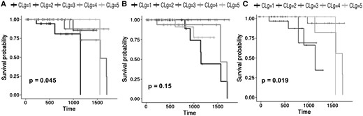
Survival curves of the BREAST dataset. (A) Survival curves of the clusters obtained with the OTRIMLE algorithm with $m^{*}$ = 2 and ${\gamma }^{*}$ = 5. (B) Survival curves obtained with the SNF algorithm with ${\alpha }^{*}=0.5$⁠. (C) survival curves obtained with the TMIX algorithm with $m^{*}$ = 2

Fig. 3.

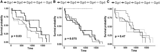
Survival curves of the LUNG dataset. (A) survival curves of the clusters obtained with the OTRIMLE algorithm by using $m^{*}$ = 11 and ${\gamma }^{*}$ = 10. (B) Survival curves obtained with the SNF algorithm with ${\alpha }^{*}=0.5$⁠. (C) Survival curves obtained with the TMIX algorithm with $m^{*}$ = 7

Interestingly the ${\text{RLED}}_{\text{min}}$ optimization also leads to a consistent choice of $m^{*}$⁠. In dimensional reduction based on PCA analysis, the scree plot is often used as a guideline to decide how many factors to retain. The analog of the latter would be the m parameter here. If there are few dominant directions along which most of the joint variability is expressed, the scree plot will typically have an elbow shape. A well-known method is to retain a number of components that appears just prior to the elbow place. The difficulty of such method is that in practice the transition towards the elbow region is often too smooth to identify a precise corner point. Therefore, this becomes usually a supervised task. In Supplementary Section S6 of the Supplementary Materials we show the distribution of the ordered eigenvalues of the R matrix compared to $m^{*}$ for all datasets. It is remarkable that the ${\text{RLED}}_{\text{min}}$ optimization almost always leads to a choice of $m^{*}$ that is in the region where the elbow takes place. The only exception is the BREAST dataset, where $m^{*}$ is chosen much smaller than the one suggested by the elbow criterion. All this supports the idea that there is restricted set of linear combinations of gene expression levels that explain: (i) most of the joint variability measured by R; (ii) these combinations can define clusters of patients with well defined survival patterns. This evidence also allows to increase computational efficiency because the m grid can be efficiently restricted to the region where the elbow takes place. Finally, a comparison of the computational time of the SNF and TMIX versus our methodology is considered. In Supplementary Section S10 of the Supplementary Materials, the computational time of SNF and TMIX methods (in term of seconds) is significantly lower than the time used by our methodology. However in Supplementary Figure S38 of the Supplementary Materials, it can be noted that the more expensive computation of the OTRIMLE algorithm is worthwhile in terms of ${\text{RLED}}_{\text{min}}$⁠. For example, for the GLIO dataset the computational time of OTRIMLE with respect to SNF is 60 times bigger and the survival separation is almost doubled. For the same dataset, with respect to TMIX, the computational time is eight times bigger and the separability is almost five times bigger. For the LUNG cancer dataset the execution times between OTRIMLE, SNF and TMIX are comparable, but in terms of separability OTRIMLE is 10 times better that TMIX and more than 5 times better than SNF. For the BREAST cancer dataset OTRIMLE is 60 times slower than SNF, but it is 6 times better in terms of ${\text{RLED}}_{\text{min}}$⁠. Moreover, OTRIMLE is 10 times slower than TMIX, but it is 1.15 times better in term of RLEDmin. For KIDNEY dataset OTRIMLE is 94 time slower than SNF, and 23 times slower than TMIX. On the other hand OTRIMLE is 1.31 and 1.06 better in terms of separability with respect to SNF and TMIX respectively.

3.1 Over-represented pathways

Once the optimal clustering in terms of ${\text{RLED}}_{\text{min}}$ is obtained, the differentially expressed genes between each cluster and all the others are identified. The analyses were performed by using the R limma package (Ritchie et al., 2015). The list of differentially expressed genes associated to each cluster was divided into the up-regulated and down-regulated genes. A pathway over-representation analysis with respect to the KEGG pathways (Kanehisa et al., 2017) was performed for each cluster and for the two separate lists of genes. This is a powerful tool for clinicians since it allows to identify the biological mechanisms characterizing each cluster with the specific effects on the genes. The analyses were conducted with the R ClusterProfiler package (Yu et al., 2012). Furthermore, the CTD database (Davis et al., 2017) was queried to check if the over-represented pathways are known to be associated to the disease. The association between a disease and a pathway is inferred by the number of genes that the pathway shares with those associated to the disease. For simplicity and space reasons, here we report only some examples of the pathways associated to Breast Cancer and Lung Cancer only. The results for the other datasets can be found in the supplementary materials.

3.1.1 Breast cancer

The pathway over-representation analysis applied to the clusters of the breast cancer dataset resulted in a total number of 163 relevant pathways, of which 157 associated to breast cancer in the CTD database. Of these 18 are associated to the first cluster (16 from down-regulated genes and 2 from up-regulated genes), 43 are associated to the second cluster (9 from down-regulated genes and 34 from up-regulated genes), 50 are associated to the third cluster (39 from down-regulated genes and 11 from up-regulated genes), 25 are associated to the fourth cluster (5 from down-regulated genes and 20 from up-regulated genes) and 27 are associated to the fifth cluster (5 from down-regulated genes and 22 from up-regulated genes). Some of the pathways showed in Figure 4, are also listed as the top associated pathways to the breast cancer on the CTD database, meaning that they contain a high number of genes that are reported in literature to be associated with the disease. For example, the Osteoclast differentiation has 15 genes associated to the breast cancer. It has been studied since breast cancer sometimes metastasises to the skeleton inducing bone degradation (Le Pape et al., 2016). Furthermore, Cell cycle is known to be associated to breast cancer and its genes can be used for diagnosis purpose at different cancer stages (Landberg and Roos, 1997). Another example is the NF-kappa B signalling pathway, whose association with breast cancer is under study since its genes are involved into the tumour existence and in treatment resistance (Shostak and Chariot, 2011). The list of pathways associated to the clusters obtained with the SNF and TMIX algorithms can be found in the supplementary materials.

Fig. 4.

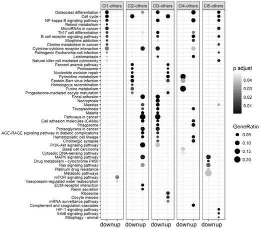
Results of the KEGG pathways over-representation analysis on the optimal clustering obtained on the BREAST cancer dataset. For each cluster the most relevant over-represented pathways from the lists of down-regulated (left column) and up-regulated (right column) genes are reported. The darker are the points in the figure, the higher is their relevance, in terms of P-values, and of the association of the pathways to the up/down regulated genes

3.1.2 Lung cancer

The pathway over-representation analysis applied to the clusters of the lung cancer dataset resulted in a total number of 76 relevant pathways, of which 75 associated to breast cancer in the CTD database. Of these 6 are associated to the first cluster (3 from down-regulated genes and 3 from up-regulated genes), 32 are associated to the second cluster (23 from down-regulated genes and 9 from up-regulated genes), 20 are associated to the third cluster (3 from down-regulated genes and 17 from up-regulated genes) and 18 are associated to the fourth cluster (15 from down-regulated genes and 3 from up-regulated genes) and 27 are associated to the fifth cluster (5 from down-regulated genes and 22 from up-regulated genes).

As shown in Figure 5 cluster 4 contains the patients that die earlier. Most of its differentially expressed genes are down-regulated and associated with pathways related to lung cancer such as Pertussis, Toxoplasmosis that can cause complications in lung cancer (Lu et al., 2015), Staphylococcus aureus infection, etc. Endocytosis is one of the pathways associated to the down regulated genes of the second cluster. It is a mechanism for cells to remove ligands, nutrients and plasma membrane (PM) proteins, and lipids from the cell surface, bringing them into the cell interior. Its pathway is associated to lung cancer by means of 8 genes on the CTD database. It is known that activating mutants of EGFR in lung cancer exploits endocytosis-related mechanisms to reduce rapid inactivation by internalization and MVB sorting, further enhancing their oncogenic properties (Polo et al., 2004). The Neuroactive ligand-receptor interaction pathway is strongly associated to the genes down regulated in cluster one and up-regulated in cluster 2. It is usually related with cancer progression (Huan et al., 2014).

Fig. 5.

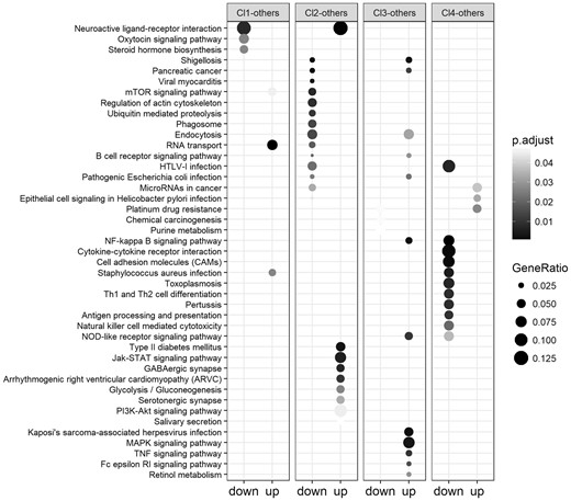
Results of the KEGG pathways over-representation analysis on the optimal clustering obtained on the LUNG cancer dataset. For each cluster the most relevant over-represented pathways from the lists of down-regulated (left column) and up-regulated (right column) genes are reported. The darker are the points in the figure, the higher is their relevance, in terms of P-values, and of the association of the pathways to the up/down regulated genes

4 Conclusion

In this study, we proposed a methodology for the analysis of gene expression data for patient sub-typing. The methodology is composed of several steps using state of the art algorithms. First the pairwise robust correlation between the genes is computed by using the RSC method. Then, the gene expression data are projected into the space composed of the first m components of the spectral decomposition. The OTRIMLE algorithm in then applied to identify robust group of patients. The survival separability of the clusters is computed in terms of the ${\text{RLED}}_{\text{min}}$ measure. Finally the differentially expressed genes of each cluster are identified and an over-representation pathway analysis is performed. We executed the experiments on five real cancer datasets and we compared our method with the SNF method, that is a state of the art approach for patient sub-typing, and with the TMIX algorithm. We showed the effectiveness of the proposed methodology by comparing the survival curves of our clusterings, in terms of separability, with those obtained with the SNF and TMIX methods. Our results suggested that the usage of measures and algorithms robust to noise allows to identify groups of patients with better survival curves even using only gene expression data instead of integrative analyses of multi-omic experiments.

Conflict of Interest: none declared.

Author notes

The authors wish it to be known that, in their opinion, the Pietro Coretto and Angela Serra authors should be regarded as Joint First Authors.