Tightly integrated genomic and epigenomic data mining using tensor decomposition

Abstract

Motivation

Complex diseases such as cancers often involve multiple types of genomic and/or epigenomic abnormalities. Rapid accumulation of multiple types of omics data demands methods for integrating the multidimensional data in order to elucidate complex relationships among different types of genomic and epigenomic abnormalities.

Results

In the present study, we propose a tightly integrated approach based on tensor decomposition. Multiple types of data, including mRNA, methylation, copy number variations and somatic mutations, are merged into a high-order tensor which is used to develop predictive models for overall survival. The weight tensors of the models are constrained using CANDECOMP/PARAFAC (CP) tensor decomposition and learned using support tensor machine regression (STR) and ridge tensor regression (RTR). The results demonstrate that the tensor decomposition based approaches can achieve better performance than the models based individual data type and the concatenation approach.

Supplementary information

Supplementary data are available at Bioinformatics online.

1 Introduction

Complex diseases such as cancers often involve multiple types of genomic and/or epigenomic abnormalities. Although mutations often are a hallmark of cancers, other types of abnormalities may also play critical roles. For example, it was discovered that copy-number amplification, rather than mutation of HER2, results in the deleterious effects of HER2 in cancer (Sanchez-Garcia et al., 2014). A recent review concluded that epigenetic changes may drive some cancers by disrupting the expression of ‘tumor progenitor genes’ (Feinberg et al., 2016). Besides, interplays between different genomic/epigenomic abnormalities may also play significant roles because one type of abnormalities may induce other types of abnormalities. For instance, DNA methylation may play a substantial role in the regulation of gene expression (Wagner et al., 2014). Therefore, comprehensive analysis by integrating various genomic and epigenomic data may provide insights into the complex nature of cancer development and progression. However, only until recent years the advances in high throughput technologies have permitted generation of significant amount of multiple types of genomic data. For instance, large scale projects such as The Cancer Genome Atlas (TCGA, https://cancergenome.nih.gov) and The International Cancer Genome Consortium (ICGC) (Hudson et al., 2010) have profiled thousands of cancer samples using multiple omics technologies such as mRNA, methylation, copy number variations and somatic mutations. Consequently, rapid accumulation of multiple types omics data demands methods for integrating the tremendous amount of multidimensional omics data in order to elucidate complex relationships among different types of genomic and epigenomic abnormalities.

1.1 Data integration methods

Current data integration approaches can be roughly divided into two groups: tight and loose approaches (Fig. 1). In a loose analysis, different type of data is utilized to build model separately (multiple models, however, may be built from one data type, such as in ensemble approaches) and the results from different models are combined afterwards in either linear, ensemble, or hierarchical manner (Ritchie et al., 2015; Thingholm et al., 2016). One simple approach is to use each model as a filter that only allows biological descriptors (e.g. genes) to pass through to next stage if defined criteria are met (e.g. statistically significant) (Holzinger and Ritchie, 2012). One major advantage of multi-staged analysis is its simplicity. However, it is not effective to reveal complex patterns from combinations of multi type data types (Ritchie et al., 2015). Moreover, different arrangements of the models may deliver different results.

Fig. 1.

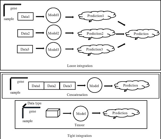
Schematic diagram for loose and tight data integration

In a tight approach, all features are combined and used to build a model or models (Ritchie et al., 2015; Thingholm et al., 2016). The simplest tight approach is to concatenate all types of data together to form a larger data matrix (Ritchie et al., 2015). For example, Mankoo et al. (Mankoo et al., 2011) concatenated copy number variation, methylation status, miRNA and gene expression data to predict time to recurrence and survival in ovarian cancer. However, the relationships between different data types are not utilized in a concatenation approach. For example, there may be correlations between mutation, copy number variation, methylation status and gene expression level (Thingholm et al., 2016). In a concatenation approach, the data of these four types are spread as four separate columns and therefore possible underlying relationships between them are disregarded. Furthermore, concatenation results in the creation of a data matrix with potentially very high dimensionality when the number of data types grows, increasing the risk of overfitting. In order to capture the relationship between different types of data, it is advantageous to organize the data in a multi-dimensional fashion.

In the present study, we propose a tightly integrated approach utilizing tensor decomposition (Kolda and Bader, 2009). Multiple types of data are arranged as a high-order tensor. One of the advantages of this approach is the number of parameters needed to be determined can be reduced, especially when the number of data types is large. Another advantage is the features associated with the same gene are organized in the same dimension, allowing discovery of possible complex patterns associated with different data types.

Tensor decomposition can be rooted back to the work by Hitchcock in 20s of the last century (Hitchcock, 1927). It has been widely used in chemometrics since early 80s (Appellof and Davidson, 1981; Smilde and Geladi, 2004) and also in other areas such as signal processing (Muti and Bourennane, 2005), and more recently graph processing (Zhou et al., 2013). Tensor decomposition has only recently found applications within bioinformatics, probably due to the lack of suitable data (Morup, 2011). For example, it was used for integrative analysis of DNA microarray data from different studies (Omberg et al., 2007). To the best of our knowledge, this study represents the first time that different types of genomic and epigenomic data are integrated using tensor structure.

2 Materials and methods

2.1 Data

The genomic, epigenomic and clinical data of TCGA ovarian serous cystadenocarcinoma (TCGA-OV) and head & neck squamous cell carcinoma (TCGA-HNSC) were downloaded from the TCGA data portal (https://gdc-portal.nci.nih.gov) and the UCSC Cancer Browser (https://genome-cancer.ucsc.edu/proj/site/hgHeatmap/), respectively. These two datasets were screened from the whole TCGA data collection because they had big sample sizes, poor survivals and each datatype was generated using a single platform (Details available in Supplementary Material). In the present study, we used gene expression (GE), DNA methylation (ME), copy number variation (CN) and somatic mutation (MU) data. In brief, the level 3 expression, methylation and copy number data of TCGA-OV were retrieved. For methylation, all probes were grouped by gene, and the maximum beta value of the all probes for a gene was assigned to this gene. Beta values, ranging from 0 to 1, represent estimated methylation levels using the ratio of intensities between methylated and unmethylated alleles. For copy number variation, the downloaded segmented CN data was mapped to genes to produce gene-level estimates. For TCGA-HNSC, instead of processing data by ourselves, we downloaded processed gene levels data from UCSC Cancer Browser. We used thresholded copy number, IlluminaHISeq percentile gene expression and Methylation450K DNA methylation data. Detailed of how these data were processed can be found at UCSC Cancer Browser website (https://genome-cancer.ucsc.edu).

2.2 Transforming somatic mutation data using network propagation

Although somatic mutations are a hallmark of cancers, the vast majority of genes in cancer cells are not mutated. Therefore, direct use of somatic mutation would result in a very sparse tensor. In this study, we utilized network propagation to integrate somatic mutations and gene interaction networks (Hofree et al., 2013; Vanunu et al., 2010). The resulting matrix is far less sparse than the input somatic mutation matrix. Besides, it contains not only somatic mutation information, but also the influence of each mutation over its network neighborhood. This method has been successfully applied to network-based stratification of tumor mutations (Hofree et al., 2013) and prioritizing disease genes (Vanunu et al., 2010).

Somatic mutation profiles of samples were firstly converted to a binary matrix based on whether a gene in a sample has a functional mutation (i.e. 1 if it has one or more of indel, nonsense, nonstop, splice site, translation start site, or missense mutations; otherwise 0). The obtained binary matrix was then projected onto human gene interaction network to generate a network propagation model using a propagation function (Vanunu et al., 2010):

$${\mathbf{F}}_{\mathbf{t}+\mathbf{1}}=\alpha {\mathbf{F}}_{\mathbf{t}}\mathbf{A}+(\mathbf{1}-\alpha ){\mathbf{F}}_0$$

(1)

where F₀ is the binary sample-by-gene mutation matrix, and A is a degree-normalized adjacency matrix of the gene interaction network. To generate the adjacency matrix, we first combined three publicly available gene/protein interaction networks, namely STRING (V.10, http://string-db.org), HumanNet (V.1, http://www.functionalnet.org/humannet/), and Pathway commons (V.8, www.pathwaycommons.org/). The combined dataset included all hits in Pathway common but only top 10% hits from HumanNet and STRING (Hofree et al., 2013). The adjacency matrix was then multiplied by a diagonal matrix with the inverse of its row sums on the diagonal to create a degree-normalized adjacency matrix. $\alpha$ is a tuning parameter that determines the distance that a mutation signal is allowed to propagate. However, the performance of the models is not sensitive to this value when the value is above 0.5 (Vanunu et al., 2010). We set the value of $\alpha$ to 0.5 in the present study. The propagation function was executed iteratively until converge, defined as F_t+1 – F_t < 1 * 10⁻⁴.

Different data types may include different sets of genes. For the present study, we only considered genes with all four data types to avoid missing data points. Overall, we obtained data for 7477 genes * 445 samples for TCGA-OV, and 13678 genes * 480 samples for TCGA-HNSC. The difference of the numbers of genes in the two datasets was largely due to the different methylation platform: Methylation27K for TCGA-OV while Methylation450K for HNSC which had significantly different numbers of probes and, therefore, coverages.

2.3 Learning algorithms

In this section, we briefly introduce the notions of tensor and tensor decomposition. Because there are many algorithms available and in practice we can only compare a few of them, we focused on the matrix-based regression algorithms using the same base algorithms, namely support vector regression (SVR) and RIDGE regression, as those used in tensor regression for direct comparison. We also included state-of-the-art regular random forests (RF) (Breiman, 2001) and random survival forests (RSF) (Ishwaran et al., 2008) algorithms to provide additional comparison.

2.3.1 Tensor

The term tensor is used to generalize vector (first-order tensor), matrices (second-order tensor) and higher-order arrays (Kolda and Bader, 2009). In the present study, third-order tensors were used to store the all genomic and epigeomic data. The three dimensions of the tensors include sample, gene and data type.

2.3.2 CANDECOMP/PARAFAC (CP) tensor decomposition

It was suggested that a tensor $\omega$ can be expressed as the sum of a finite number of rank-one tensors (Kolda and Bader, 2009). The rank of the tensor is the smallest number of rank-one tensors that generate $\omega$ as their sum. An N-order tensor is rank-one if it equals to the outer product of N vectors. The procedure is often termed as the CANDECOMP/PARAFAC (CP) decomposition, which factorizes a tensor into a sum of R component rank-one tensors (Kolda and Bader, 2009):

$$\mathbf{\omega }\approx \sum _{\mathrm{r}=1}^{\mathrm{R}}{\mathbf{u}}_{\mathrm{r}}^{\left(1\right)}\mathrm{ }\mathrm{o}\mathrm{ }{\mathbf{u}}_{\mathrm{r}}^{\left(2\right)}\dots \mathrm{o}\mathrm{ }{\mathbf{u}}_{\mathrm{r}}^{\left(\mathrm{M}\right)}$$

(2)

where R is the rank of the CP decomposition, M is the order of the tensor and the symbol ‘o’ represents the vector outer product.

2.3.3 Tensor learning model

Linear tensor learning models in the present study were generalized from the conventional vector linear model as (Guo et al., 2012):

$$\mathrm{y}=\mathrm{f}\left(\mathbf{\chi };\mathbf{\omega },\mathrm{b}\right)=〈\mathbf{\chi },\mathbf{\omega }〉+\mathrm{b}$$

(3)

where χ$\mathrm{ }\in {\mathrm{I}\mathrm{R}}^{{\mathrm{I}}_1\mathrm{*}\mathrm{ }{\mathrm{I}}_2\dots \mathrm{*}{\mathrm{I}}_{\mathrm{M}}}$ is the input tensor, ω is the weight tensor in the same dimension as χ, y is the regression outcome, f represents regression function, and scalar b is the bias of the model. The learning process is to determine the weight tensor and bias based on the training data. The number of parameters needed to be learned is equal to ${\mathrm{I}}_1\mathrm{*}\mathrm{ }{\mathrm{I}}_2..\mathrm{*}{\mathrm{I}}_{\mathrm{M}}$ (i.e. ${\prod }_{\mathrm{k}\hspace{0.17em}=\hspace{0.17em}1}^{\mathrm{M}}{\mathrm{I}}_{\mathrm{k}}$ where M is the order of the tensor). Thus, when M is high, the number of weights can be significant; consequently, overfitting and other problems associated with high computational complexity may appear. This can be especially problematic when the number of cases to learn parameters from is small, relative to the number of available training cases. In this study, we used the CP algorithm to constrain the weight tensor $\omega$ to a sum of R component rank-one tensors (Eq. 4). This approach reduces the number of parameters that need to be estimated from ${\prod }_{\mathrm{k}\hspace{0.17em}=\hspace{0.17em}1}^{\mathrm{M}}{\mathrm{I}}_{\mathrm{k}}$ to R${\sum }_{\mathrm{k}\hspace{0.17em}=\hspace{0.17em}1}^{\mathrm{M}}{\mathrm{I}}_{\mathrm{k}}$⁠.

(4)

where ‘o’ represents the vector outer product. The weight matrix and bias were trained from a set of training data using support tensor regression (STR) and RIDGE tensor regression (RTR) (Guo et al., 2012). As their names indicated, STR and RTR are expansions of support vector machine and RIDGE regression, respectively.

In most cases, it is difficult to determine the exact rank of a tensor because it is a NP-hard problem (Håstad, 1990). Thus, in practice the rank is usually determined by fitting multiple CP decomposition with different ranks until a reasonably ‘good’ rank is found. For each possible R to test, a common method to compute the CP decomposition of a tensor is the alternating least squares (ALS) method, which only optimize one mode at a time while all other modes are fixed (Kolda and Bader, 2009).

To achieve unbiased estimate of the performance of predictive models in the study, we used a nested cross validation (CV) procedure (Varma and Simon, 2006). In brief, the inner CV was used to conduct a parameter search of the STR or RTR parameters and the outer CV was used to measure the performance of the model based on parameters determined in the inner CV. Because the external fold used in the outer CV was never seen in the inner model selection, the nested CV is considered to provide unbiased estimate of the true error (Varma and Simon, 2006). For simplicity and consistency, we only considered linear models which used the same parameter set (relative weight of the regularization term C = 2^[−5, −3, −1, 1,…, 17, 19]) in inner CV for all tensor and matrix based models. The TCGA data are vulnerable to batch effects because the tumor samples that the data were derived upon were collected and processed in different institutions at different times (Leek et al., 2010). To achieve realistic estimate of performance, we adopted a leave-one-batch-out (LOBO) CV procedure in which all data from one batch were grouped and used as training or test data together (Varma and Simon, 2006).

2.4 Performance evaluation

To evaluate the performance of the models, we combined all predictions from the outer CV and calculated its concordance index (C-index). C-index is the fraction of all pairs of subjects whose observed survival times are correctly ordered by the predictive model. It is considered as a ‘global’ index for estimating the predictive ability of a survival model. We then divided all subjects equally into two groups, namely higher risk and lower risk groups, based on predicted survival times. We created Kaplan-Meier estimators to evaluate the statistical significance of the difference between these two groups (Kaplan and Meier, 1958). In addition, we developed Cox models to calculate the hazard ratios (HR) and their associated P-values of the higher and lower risk groups (Cox, 1972). We also reported the mean, 3-year and 5-year survivals for both groups.

3 Results

3.1 Predictive models using single type of genomic data

To evaluate how informative each type of genomic and epigenomic data is, and to perform direct comparison with the tensor based models we planned to develop, we first built SVR and RIDGE regression models using GE, ME, CN and MU data sets separately. We optimized the parameters using the inner CV and then built testing models in the outer CV to estimate the performance of these SVR models. The numeric metrics of the models are summarized in Table 1 and their Kaplan-Meier curves are available in Supplementary Table S1. Among all four data types, GE was the only one that resulted in models with statistically significant differences between higher and lower risk groups for both datasets. Other data types lead to models with little to modest prediction power except methylation data that achieved significant separation for TCGA-OV (P-value: 0.0483) used in SVR models. The trend can be consistently seen in hazard ratio, C-Index, 3- and 5-year survivals.

Table 1.

Performance of matrix based models

		TCGA-OV				TCGA-HNSC
		SVR	RIDGE	RF	RSF	SVR	RIDGE	RF	RSF
GE	C-index	0.581	0.584	0.523	0.488	0.553	0.586	0.583	0.496
	HR (P-value)	1.52 (1.74e−3)	1.29 (0.0577)	0.886 (0.372)	0.869 (0.298)	1.45 (1.31e−2)	1.54 (4.16e−3)	1.68 (6.1e−4)	0.968 (0.829)
	Median	38.6/50.4	38.6/50	45.8/45.4	48.2/44.5	36.3/68.3	37.8/58.7	37.8/68.8	53/58.7
	3Y Survival	0.554/0.717	0.552/0.717	0.627/0.652	0.648/0.629	0.507/0.664	0.511/0.671	0.523/0.66	0.577/0.607
	5Y Survival	0.251/0.382	0.283/0.354	0.357/0.295	0.255/0.373	0.402/0.528	0.437/0.493	0.416/0.521	0.459/0.479
ME	C-index	0.561	0.553	0.509	0.508	0.527	0.521	0.493	0.487
	HR (P-value)	1.3 (0.0483)	1.16 (0.275)	0.85 (0.227)	0.862 (0.271)	1.05 (0.728)	1.01 (0.921)	0.852 (0.285)	0.919 (0.569)
	Median	41/49	42/49.4	49/44.9	48.2/44.1	58.3/53	58.3/54.7	58.2/48.9	65.7/57.3
	3Y Survival	0.59/0.686	0.608/0.669	0.65/0.629	0.652/0.625	0.576/0.603	0.588/0.59	0.611/0.566	0.587/0.591
	5Y Survival	0.298/0.341	0.307/0.336	0.368/0.272	0.346/0.284	0.471/0.454	0.458/0.476	0.496/0.436	0.504/0.434
CN	C-index	0.528	0.57	0.43	0.425	0.521	0.467	0.503	0.504
	HR (P-value)	1.11 (0.442)	1.39 (0.0145)	0.725 (1.61e−2)	0.715 (1.16e−2)	1.13 (0.427)	0.847 (0.263)	1.01 (0.965)	0.96 (0.783)
	Median	42.1/49	38.8/52.6	49.5/41.6	49.7/39.7	48.9/58.3	57.3/57.7	48.9/68.8	58.3/53
	3Y Survival	0.601/0.68	0.57/0.707	0.701/0.578	0.707/0.573	0.576/0.603	0.62/0.556	0.603/0.573	0.605/0.571
	5Y Survival	0.292/0.35	0.266/0.375	0.377/0.263	0.378/0.264	0.435/0.497	0.47/0.461	0.434/0.511	0.499/0.436
MU	C-index	0.561	0.488	0.58	0.587	0.502	0.506	0.551	0.541
	HR (P-value)	1.2 (0.164)	0.974 (0.844)	1.43 (6.89e−3)	1.56 (9.52e−4)	0.89 (0.433)	0.866 (0.332)	1.18 (0.272)	1.18 (0.267)
	Median	39.6/48.2	48.2/44.1	41/49.7	38.9/52.6	57.7/53	58.3/53	57.3/57.7	54.7/61.3
	3Y Survival	0.583/0.697	0.621/0.659	0.557/0.725	0.541/0.741	0.625/0.558	0.606/0.571	0.552/0.626	0.55/0.631
	5Y Survival	0.3/0.343	0.35/0.294	0.266/0.375	0.247/0.396	0.453/0.476	0.495/0.442	0.463/0.462	0.435/0.507
All	C-index	0.577	0.561	0.575	0.508	0.553	0.551	0.584	0.536
	HR (P-value)	1.43(7.93e−3)	1.26 (0.0801)	1.26 (0.0806)	0.862 (0.271)	1.45 (1.31e−2)	1.23 (0.157)	1.68 (5.82e−4)	1.23 (0.171)
	Median	38.9/52.1	41.6/49	41/49	48.2/44.1	36.3/68.8	46.6/66.7	37.8/68.8	48.6/61.3
	3Y Survival	0.578/0.695	0.585/0.693	0.573/0.707	0.652/0.625	0.507/0.664	0.547/0.635	0.513/0.667	0548/0.638
	5Y Survival	0.246/0.387	0.304/0.338	0.301/0.34	0.346/0.284	0.402/0.528	0.409/0.53	0.409/0.525	0.427/0.519

All, concatenated data; C-index, concordance index; HR, hazard ratio of higher risk group and lower risk groups; Median, median survival (months) of higher risk group/lower risk group; 3Y (5Y) survival, three (five) year survival of higher risk group/lower risk group; SVR, support vector regression; RIDGE, RIDGE regression; RF, random forest regression; RSF, random survival forests regression.

In addition to SVR and RIDGE regression, we also developed RF and RSF regression models using individual and concatenated datasets (Table 1). While GE afforded the best performance model with individual data for HNSC, MU delivered the most predictive model for TCGA-OV dataset, suggesting network propagation resulted in informative transformed data. Interestingly, RF and RSF gave different performance for TCGA-OV and TCGA-HNSC datasets: while RFS in general out-performed RF for the TCGA-OV data, overall RF was the better choice for TCGA-HNSC.

3.2 Predictive models using concatenated genomic data

One simple way to integrate a number of genomic and epigenomic data is to concatenate all data types to form a large data matrix with the size of n * ${\sum }_{k=1}^M{I}_k$ where n is the number of cases, M is the number of data types and I_k is the number of features for the data type k. To compare the concatenation approach with the proposed tensor based data integration, we developed SVR and RIDGE models using concatenated features. In the present study, there are 4*7477 features for TCGA-OV, and 4*13678 features for TCGA-HNSC. We used the same nested CV to select the parameters and estimate the performance. The performance of the SVR model is very similar to the SVR model using GE features (Table 1). Consistent with the previous findings that SVR has strong tolerance against noise contamination (Raymond et al., 2017).

3.3 Tensor based predictive models

We developed a series of STR models for TCGA-OV and TCGA-HNSC with rank = 1, 2, 3 (Table 2 and Fig. 2). All models delivered Kaplan-Meier curves that showed statistical difference between higher and lower risk groups. For TCGA-OV, the rank2 model delivered the best separation while rank3 model delivered the best results for TCGA-HNSC. Therefore, the optimal rank may depend on the characteristics of the data. The number of features used in tensor models, as well as the numbers for concatenation models are summarized in Table 3. It is noteworthy that the rank1 models for both data sets delivered better performance than GE alone and concatenated models while only including approximate one fourth of features of the concatenated model.

Table 2.

Performance of tensor based models

	Rank	Metrics	TCGA-OV	TCGA-HNSC
STR	1	C-index	0.573	0.589
		HR (P-value)	1.55 (1.1e−3)	1.71 (3.56e−4)
		Median	39.6/50.4	32.8/77.3
		3Y Survival	0.57/0.707	0.499/0.673
		5Y survival	0.257/0.385	0.387/0.543
	2	C-index	0.594	0.566
		HR (P-value)	1.61 (3.75e−4)	1.59 (1.8e−4)
		Median	39.6/52.6/	37.8/77.3
		3Y Survival	0.579/0.697	0.514/0.658
		5Y survival	0.239/0.396	0.381/0.545
	3	C-index	0.585	0.563
		HR (P-value)	1.44 (6.17e−3)	1.72 (2.86e−4)
		Median	41/50	33.1/90.1
		3Y Survival	0.588/0.688	0.495/0.675
		5Y survival	0.262/0.375	0.367/0.556
RTR	1	C-index	0.582	0.553
		HR (P-value)	1.44 (6.17e−3)	1.53 (3.9e−3)
		Median	39.9/50	37.8/68.8
		3Y Survival	0.579/0.698	0.514/0.658
		5Y survival	0.265/0.373	0.392/0.535
	2	C-index	0.611	0.576
		HR (P-value)	1.65 (1.77e−4)	1.63 (1.03e−3)
		Median	38.5/50.4	37.8/68.8
		3Y Survival	0.547/0.728	0.527/0.651
		5Y survival	0.387/0.252	0.3910.542

STR, support tensor regression; RTR, RIDGE tensor regression; C-index, concordance index; HR, hazard ratio of higher risk and lower risk groups; Median, median survival (months) of higher risk group/lower risk group; 3Y (5Y) survival, three (five) year survival of higher risk group/lower risk group.

Table 3.

Numbers of features used in the models

	Tensor			Matrix
	Rank1	Rank2	Rank3	Concatenation
OV	7481	14962	22443	29908
HNSC	13682	27364	41046	54712

Fig. 2.

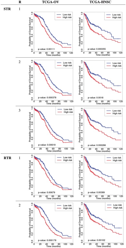
Kaplan-Meier curves of tensor-based models. R, rank; STR, support tensor regression; RTR, RIDGE tensor regression

We then attempted to build RTR models for TCGA-OV and TCGA-HNSC (Table 2 and Fig. 2). However, we were only able to build ranks 1 and 2 because rank3 models were very time consuming and we were not able to build all models within a reasonable time frame. For both datasets, rank2 models performed better than rank1. Overall, STR and RTR models delivered similar performance.

Comparing tensor based models with matrix based models, it is clear that the best performance scores were usually associated with tensor models. For example, For TCGA-OV dataset, the best C-index is 0.611 for tensor based models (RTR Rank2) versus 0.587 (RFS model for MU data) for matrix based models, and best HR (P-value) is 1.65 (1.77e−4) for the RTR Rank2 model versus 1.56 (9.52e−4) for the RFS model of MU data. The same trend can be found for other metrics and the TCGA-HNSC dataset (Tables 1 and 2).

3.4 Computational complexity and execution time

In this section, we compare empirical execution times of the tensor based approach with the concatenation method. There are two different types of computational complexity and execution time involved in most machine learning based predictive model development: at training time and at test time. The computational complexity at the test time for tensor decomposition based approach is linear to the overall number of features, so as the concatenation based approach. Therefore, there is no significant difference between these two approaches. The training time computational complexity and execution time are more difficult to estimate. However, the base operations of tensor based approaches are the linear SVR or RIDGE regressions, same as the concatenation approach, because the ALS method optimizes one mode at a time. Although the total number of features are identical, all features in the concatenated approach are in the same matrix while the features in the tensor approach are arranged in three dimensions. Thus, it takes more time to build a model using concatenation than tensor approaches. The tensor approach, however, often requires multiple iterations. The number of iterations is determined by the nature of the data and is impossible to predict. Thus, we only report the average empirical time to build the outer CV models of the tensor and matrix based approaches for both TCGA-OV and TCGA-HNSC datasets (Table 4). Overall, TCGA-HNSC model requires more time than its TCGA-OV counterpart because the former has more features. Higher-rank models demand more time than lower-rank models. In fact, we were not able to complete rank3 RTR models within reasonable time frame. Interestingly, the Rank 1 and 2 STR model building is slower than the concatenation models while the rank 1 and 2 RTR model building is faster than the corresponding concatenated matrix model building. However, the required time increases rapidly with the rank; consequently, it was not feasible to build rank3 RTR models within a reasonable time frame. For STR models, even though Rank1 and Rank2 models requires more time than the concatenation approach, the time increases relatively slowly with the rank. As a consequence, we were able to build rank3 STR models. Taken together, apparently, RTR has advantages at lower rank, but STR may be the choice for higher rank CP decomposition when necessary.

Table 4.

Average execution time (in minutes) for one outer CV training run

		Tensor			Matrix
		Rank1	Rank2	Rank3	Concatenation
STR	OV	16	19	34	13
	HNSC	43	239	408	16
RTR	OV	13	89	NA	106
	HNSC	50	539	NA	602

Note: All jobs were executed in a computer system with 128 cores (2.27 GHz 8-core Xeon™ X7560) and 1 TB of memory. STR: support tensor regression; RTR: RIDGE tensor regression.

4 Discussion and conclusions

As we discussed in the previous sections, CP tensor decomposition based models require fewer parameters while preserving underlying relationship among different data types, compared to concatenated models (Table 3). In general, it reduces the number of parameters that need to be estimated from ${\prod }_{\mathrm{k}\hspace{0.17em}=\hspace{0.17em}1}^{\mathrm{M}}{\mathrm{I}}_{\mathrm{k}}$ to R${\sum }_{\mathrm{k}\hspace{0.17em}=\hspace{0.17em}1}^{\mathrm{M}}{\mathrm{I}}_{\mathrm{k}}$⁠. Currently we used four different types of features in the present study. It is reasonable to believe the reduction can be more significant when more types of data and, perhaps even more important, additional dimensions such as time series data become available.

Tensor approach comes with some drawbacks. For example, CP decomposition requires the set of matrices have the same numbers of rows and columns to be modeled as a tensor. Genes are the best vehicle to organize features as many genomic and epigenomic features can be directly associated with genes. However, some genomic or epigenomic features cannot be easily mapped to genes. For example, currently the reported number of microRNA is only a few thousands (Kozomara and Griffiths-Jones, 2011). Nevertheless, a microRNA functions by regulating its targeted genes. Therefore, the impact of microRNA can be modeled at the gene level by considering its impact to individual genes, similar to the way that we transformed the mutation data in this study. Currently we are exploring such an approach. In addition, algorithm such as PARAFAC2 can be applied to a collection of matrices that each have the same number of columns but a different number of rows (Helwig, 2017). Alternatively, multiple tensors can be used to model complex data at multiple levels (Khan et al., 2016), e.g. one for DNA and another for microRNA. Moreover, curated data such as pathway structure can also be considered to further improve performance and learn biological structures (Zhang et al., 2017). Applications of these algorithms in genomic and epigenomic data will be investigated separately. We also invite the research community to conduct research in this promising area.

In the present study, we did not allow missing data in the tensor, which resulted in filtering a number of genes, especially for TCGA-OV dataset. This was largely due to the low coverage of the Methylation27K platform used to generate the methylation data. We expect the number of missing genes will be much smaller for newer datasets because sequencing based genomic and epi-genomic data have become increasingly popular. Besides, methodologies designed for tensor decomposition with missing data can be employed (Acar et al., 2010; Khan and Kaski, 2014). It is possible to impute missing data using various algorithms (Sterne et al., 2009); cautions should be taken, however, because imputation may introduce biases and therefore is not suitable for all datasets. In the present study we did not apply imputation to avoid additional complexity.

The present study should be considered as the first step toward modeling complex genomic and epigenomic data using the tensor structure. For example, we did not attempt to determine the true rank of the tensors, despite that it is crucially important for most studies. Recent development of algorithms that can be used to automatically determine the rank of tensors may overcome the computational burden to determine the true rank of tensors (Khan and Kaski, 2014). We only focused on lower rank decomposition in the present study; it should be pointed out, however, it can be very useful to study higher ranks. Thus, further optimization of the rank may yield better results and provide valuable insight into underlying biological structures.

In summary, we have presented a proof-of-the-concept study using tensor to model genomic and epigenomic data. It is encouraging that the results have clearly demonstrated the feasibility and the models have achieved better performance than single data type and concatenated approaches. Currently we are actively exploring feature selection algorithms to identify informative features and elucidate the complex interrelationships to take the advantage of tensor based modeling, which will allow discovery of biological structures relevant to disease prognosis and treatment.

Acknowledgements

We wish to thank the two anonymous reviewers and the editor for their constructive comments and suggestions. We are grateful to Drs. Joanna Shih, Julia Krushkal Adkins, Yingdong Zhao, and Yongcui Wang for valuable suggestions and comments. This work utilized the computational resources of the NIH HPC Biowulf cluster (http://hpc.nih.gov). The results shown here are in whole or part based upon data generated by the TCGA Research Network: http://cancergenome.nih.gov/.

Conflict of Interest: none declared.

Disclaimer: The views expressed in this article are the personal opinions of the authors and do not necessarily reflect policy of the US National Cancer Institute.