Block HSIC Lasso: model-free biomarker detection for ultra-high dimensional data

Abstract

Motivation

Finding non-linear relationships between biomolecules and a biological outcome is computationally expensive and statistically challenging. Existing methods have important drawbacks, including among others lack of parsimony, non-convexity and computational overhead. Here we propose block HSIC Lasso, a non-linear feature selector that does not present the previous drawbacks.

Results

We compare block HSIC Lasso to other state-of-the-art feature selection techniques in both synthetic and real data, including experiments over three common types of genomic data: gene-expression microarrays, single-cell RNA sequencing and genome-wide association studies. In all cases, we observe that features selected by block HSIC Lasso retain more information about the underlying biology than those selected by other techniques. As a proof of concept, we applied block HSIC Lasso to a single-cell RNA sequencing experiment on mouse hippocampus. We discovered that many genes linked in the past to brain development and function are involved in the biological differences between the types of neurons.

Availability and implementation

Block HSIC Lasso is implemented in the Python 2/3 package pyHSICLasso, available on PyPI. Source code is available on GitHub (https://github.com/riken-aip/pyHSICLasso).

Supplementary information

Supplementary data are available at Bioinformatics online.

1 Introduction

Biomarker discovery, the goal of many bioinformatics experiments, aims at identifying a few key biomolecules that explain most of an observed phenotype. Without a strong prior hypothesis, these molecular markers have to be identified from data generated by high-throughput technologies. Unfortunately, finding relevant molecules is a combinatorial problem: for d features, $2^d$ binary choices must be considered. As the number of features vastly exceeds the number of samples, biomarker discovery is a high-dimensional problem. The statistical challenges posed by such high-dimensional spaces have been thoroughly reviewed elsewhere (Clarke et al., 2008; Johnstone and Titterington, 2009). In general, due to the curse of dimensionality, fitting models in many dimensions and on a small number of samples is extremely hard. Moreover, since biology is complex, a simple statistical model such as a linear regression might not be able to find important biomarkers. Those that are found in such experiments are often hard to reproduce, suggesting overfitting. Exploring the solution space and finding true biomarkers are not only statistically challenging, but also computationally expensive.

In machine learning terms, biomarker discovery can be formulated as a problem of feature selection: identifying the best subset of features to separate between categories, or to predict a continuous response. In the past decades, many feature selection algorithms that deal with high-dimensional datasets have been proposed. Due to the difficulties posed by high-dimensionality, linear methods tend to be the feature selector of choice in bioinformatics. A widely used linear feature selector is the Least Absolute Shrinkage and Selection Operator, or Lasso (Tibshirani, 1996). Lasso fits a linear model between the input features and phenotype by minimizing the sum of the least square loss and an ${\ell }_1$ penalty term. The balance between the least square loss and the penalty ensures that the model explains the linear combination of features, while keeping the number of features in the model small. However, in many instances biological phenomena do not behave linearly. In such cases, there is no guarantee that Lasso can capture those non-linear relationships or an appropriate effect size to represent them.

In the past decade, several non-linear feature selection algorithms for high-dimensional datasets have been proposed. One of the most widely used, called Sparse Additive Model, or SpAM (Ravikumar et al., 2009), models the outcome as a sparse linear combination of non-linear functions based on kernels. However, since SpAM assumes an additive model over the selected features, it cannot select important features if the phenotype cannot be represented by the additive functions of input features—for example, if there exist a multiplicative relationship between features (Yamada et al., 2014).

Another family of non-linear feature selectors are association-based: they compute the statistical association score between each input feature and the outcome, and rank features accordingly. Since these approaches do not assume any model about the output, they can detect important features as long as an association exists. When using a non-linear association measure, such as the mutual information (Cover and Thomas, 2006) or the Hilbert–Schmidt Independence Criterion (HSIC) (Gretton et al., 2005), they select the features with the strongest dependence with the phenotype. However, association-based methods do not account for the redundancy between the features, which is frequent in biological datasets, since they do not model relationships between features. Hence, many redundant features are typically selected, hindering interpretability. This is important in applications like drug target discovery, where only a small number of targets can be validated, and it is crucial to discriminate the most important target out of many other top-ranked targets.

To deal with the problem of redundant features, Peng et al. (2005) proposed the minimum redundancy maximum relevance (mRMR) algorithm. mRMR can select a set of non-redundant features that have high association to the phenotype, while penalizing the selection of mutually dependent features. Ding and Peng (2005) used mRMR to extract biomarkers from microarray data, finding that the selected genes captured better the variability in the phenotypes than those identified by state-of-the-art approaches. However, mRMR has three main drawbacks: the optimization problem is discrete; it must be solved by a greedy approach and the mutual information estimation is difficult (Walters-Williams and Li, 2009). Moreover, it is unknown whether the objective function of mRMR has good theoretical properties such as submodularity (Fujishige, 2005), which would guarantee the optimality of the solution.

Recently, Yamada et al. (2014) proposed a kernel-based mRMR algorithm called HSIC Lasso. Instead of mutual information, HSIC Lasso employs the HSIC (Gretton et al., 2005) to measure dependency between variables. In addition, it uses an ${\ell }_1$ penalty term to select a small number of features. This results in a convex optimization problem, for which one can therefore find a globally optimal solution. In practice, HSIC Lasso has been found to outperform mRMR in several experimental settings (Yamada et al., 2014). However, HSIC Lasso is memory intensive: its memory complexity is $O(d{n}^2)$⁠, where d is the number of features and n is the number of samples. Hence, HSIC Lasso cannot be applied to datasets with thousands of samples, nowadays widespread in biology. A MapReduce version of HSIC Lasso has been proposed to address this drawback, and it is able to select features in ultra-high dimensional settings (10⁶ features, 10⁴ samples) in a matter of hours (Yamada et al., 2018). However, it requires a large number of computing nodes, inaccessible to common laboratories. Since it relies on the Nyström approximation of Gram matrices (Schölkopf and Smola, 2002), the final optimization problem is no longer convex, and hence finding a globally optimal solution cannot be easily guaranteed.

In this article, we propose block HSIC Lasso: a simple yet effective non-linear feature selection algorithm based on HSIC Lasso. The key idea is to use the recently proposed block HSIC estimator (Zhang et al., 2018) to estimate the HSIC terms. By splitting the data in blocks of size $B\ll n$⁠, the memory complexity of HSIC Lasso goes from $O(d{n}^2)$ down to $O(\mathit{dnB})$⁠. Moreover the optimization problem of the block HSIC Lasso remains convex. Through its application to synthetic data and biological datasets, we show that block HSIC Lasso can be applied to a variety of settings and compares favorably with the vanilla HSIC Lasso algorithm and other feature selection approaches, linear and non-linear, as it selects features more informative of the biological outcome. Further considerations on the state of the art and the relevance of block HSIC Lasso can be found in Supplementary File 1.

2 Materials and methods

2.1 Problem formulation

Assume a dataset with n samples described by d real-valued features, each corresponding to a biomolecule (e.g. the expression of one transcript, or the number of major alleles observed at a given SNP), and a label, continuous or binary, describing the outcome of interest (e.g. the abundance of a target protein, or disease status). We denote the ith sample by ${\mathit{x}}_i={[x_i^{(1)},x_i^{(2)},\dots ,x_i^{(d)}]}^{\top }\in {\mathbb{R}}^d$⁠, where $\top$ denotes transpose; and its label by $y_i\in \mathcal{Y}$⁠, where $\mathcal{Y}=\{0,1\}$ for a binary outcome, corresponding to a classification problem, and $\mathcal{Y}=\mathbb{R}$ for a continuous outcome, corresponding to a regression problem. In addition, we denote by ${\mathit{f}}_k={[x_1^{(k)},x_2^{(k)},\dots ,x_n^{(k)}]}^{\top }\in {\mathbb{R}}^n$ the kth feature in the data.

The goal of supervised feature selection is to find m features (⁠$m\ll d$⁠) that are the most relevant for predicting the output y for a sample $\mathit{x}$⁠.

2.2 HSIC Lasso

Measuring the dependence between two random variables X and Y can be achieved by the HSIC (Gretton et al., 2005):

$$\begin{array}{c}\text{HSIC}(X,Y)\hspace{0.17em}={\mathbb{E}}_{x,x\prime ,y,y\prime }[K(x,x\prime )L(y,y\prime )]\\ \hspace{1em}\hspace{1em}\hspace{1em}\hspace{1em}\hspace{1em}+{\mathbb{E}}_{x,x\prime }[K(x,x\prime )]{\mathbb{E}}_{y,y\prime }[L(y,y\prime )]\\ \hspace{1em}\hspace{1em}\hspace{1em}\hspace{1em}\hspace{1em}\hspace{1em}\hspace{0.17em}-2{\mathbb{E}}_{x,y}\left[{\mathbb{E}}_{x\prime }[K(x,x\prime )]{\mathbb{E}}_{y\prime }[L(y,y\prime )]\right],\end{array}$$

(1)

where $K:{\mathbb{R}}^d\times {\mathbb{R}}^d\to \mathbb{R}$ and $L:\mathcal{Y}\times \mathcal{Y}\to \mathbb{R}$ are positive definite kernels, and ${\mathbb{E}}_{x,x\prime ,y,y\prime }$ denotes the expectation over independent pairs (x, y) and $(x\prime ,y\prime )$ drawn from p(x, y). $\text{HSIC}(X,Y)$ is equal to 0 if X and Y are independent, and is non-negative otherwise.

In practice, for a given Gram matrix ${\mathit{K}}_k\in {\mathbb{R}}^{n\times n}$⁠, computed from the kth feature, and a given output Gram matrix $\mathit{L}\in {\mathbb{R}}^{n\times n}$⁠, the normalized variant of HSIC is computed using its V-statistic estimator as (Yamada et al., 2018)

$${\text{HSIC}}_v({\mathit{f}}_k,\mathit{y})=\text{tr}(\overline{{\mathit{K}}_k}\hspace{0.17em}\overline{\mathit{L}}),$$

(2)

where for a Gram matrix $\mathit{K}\in {\mathbb{R}}^{n\times n},\hspace{0.17em}\overline{\mathit{K}}$ is defined as $\overline{\mathit{K}}=\mathit{HKH}/\left|\right|\mathit{HKH}|{|}_F$ with $\mathit{H}\in {\mathbb{R}}^{n\times n}$ a centering matrix defined by $H_{\mathit{ij}}={\delta }_{\mathit{ij}}-\frac{1}{n}$⁠. Here δ_ij is equal to 1 if i = j and 0 otherwise, and $\text{tr}$ denotes the trace. Note that we employ the normalized variant of the original empirical HSIC.

The largest the value of ${\text{HSIC}}_v({\mathit{f}}_k,\mathit{y})$⁠, and the more dependent the kth feature and the outcome are. Song et al. (2012) therefore proposed to perform feature selection by ranking the features by descending value of ${\text{HSIC}}_v({\mathit{f}}_k,\mathit{y})$⁠.

With HSIC Lasso, Yamada et al. (2014) extend the work of Song et al. (2012) so as to avoid selecting multiple redundant features. For this purpose, they introduce a vector $\mathit{\alpha }={[{\alpha }_1,\dots ,{\alpha }_d]}^{\top }$ of feature weights and solve the following optimization problem:

$$\underset{\mathit{\alpha }\ge 0}{\max }\sum _{k=1}^d{\alpha }_k{\text{HSIC}}_v({\mathit{f}}_k,\mathit{y})-\frac{1}{2}\sum _{k,k\prime =1}^d{\alpha }_k{\alpha }_{k\prime }{\text{HSIC}}_v({\mathit{f}}_k,{\mathit{f}}_{k\prime })-\lambda \left|\right|\mathit{\alpha }|{|}_1.$$

(3)

The first term enforces selected features that are highly dependent on the phenotype; the second term penalizes selecting mutually dependent features and the third term enforces selecting a small number of features. The selected features are those that have a non-zero coefficient α_k. Here $\lambda >0$ is a regularization parameter that controls the sparsity of the solution: the larger λ, the fewer features have a non-zero coefficient.

The HSIC Lasso optimization problem can be rewritten as

$$\underset{\mathit{\alpha }\ge 0}{\min }\hspace{0.17em}\left|\right|\text{vec}(\overline{\mathit{L}})-[\text{vec}({\overline{\mathit{K}}}_1),\dots ,\text{vec}({\overline{\mathit{K}}}_d)]\mathit{\alpha }|{|}_2^2+\lambda |\left|\mathit{\alpha }\right|{|}_1,$$

where $\text{vec}:{\mathbb{R}}^{n\times n}\to {\mathbb{R}}^{n^2},\mathit{K}\mapsto [K_{11},\dots ,K_{1n},K_{21},\dots ,K_{\mathit{nn}}]$ is the vectorization operator. Using this formulation, we can solve the problem using an off-the-shelf non-negative Lasso solver.

HSIC Lasso performs well for high-dimensional data. However, it requires a large memory space (⁠$O(d{n}^2)$⁠), since it stores d Gram matrices. To handle this issue, two approximation methods have been proposed. The first approach uses a memory lookup to dramatically reduce the memory space (Yamada et al., 2014). However, since this method needs to perform a large number of memory lookups, it is computationally expensive. Another approach (Yamada et al., 2018) is to rewrite the problem using the Nyström approximation (Schölkopf and Smola, 2002) and solve the problem using a cluster. However using the Nyström approximation makes the problem non-convex.

2.3 Block HSIC Lasso

In this article, we propose an alternative HSIC Lasso method for large-scale problems, the block HSIC Lasso, which is convex and can be efficiently solved on a reasonably sized server.

Block HSIC Lasso employs the block HSIC estimator (Zhang et al., 2018) instead of the V-statistics estimator of Equation (2). More specifically, to compute the block HSIC, we first partition the training dataset into $n/B$ partitions ${\left\{{\{({\mathit{x}}_i^{\ell },y_i^{\ell })\}}_{i=1}^B\right\}}_{\ell =1}^{n/B}$⁠, where B is the number of samples in each block. Note that the block size B is set to a relatively small number such as 10 or 20 (⁠$B\ll n$⁠). Then, the block HSIC estimator can be written as

$${\text{HSIC}}_b({\mathit{f}}_k,\mathit{y})=\frac{B}{n}\sum _{\ell =1}^{n/B}{\text{HSIC}}_v({\mathit{f}}_k^{(\ell )},{\mathit{y}}^{(\ell )}),$$

where ${\mathit{f}}_k^{(\ell )}\in {\mathbb{R}}^B$ represents the kth feature vector of the $\ell$th partition. Note that the computation of ${\text{HSIC}}_v({\mathit{f}}_k^{(\ell )},{\mathit{y}}^{(\ell )})$ requires $O(B^2)$ memory space. Therefore, the required memory for the block HSIC estimator is $O(n{B}^2)$⁠, where $\mathit{nB}\ll n^2$⁠.

If we denote by ${\overline{\mathit{K}}}_k^{(\ell )}\in {\mathbb{R}}^{B\times B}$ the restriction of ${\overline{\mathit{K}}}_k$ to the $\ell$th partition, and by ${\overline{\mathit{L}}}^{(\ell )}\in {\mathbb{R}}^{B\times B}$ the restriction of $\mathit{L}$ to the $\ell$th partition, then

$${\text{HSIC}}_v\left({\mathit{f}}_k^{(\ell )},{\mathit{y}}^{(\ell )}\right)=\text{tr}\left({\overline{\mathit{K}}}_k^{(\ell )}\hspace{0.17em}{\overline{\mathit{L}}}^{(\ell )}\right)=\text{vec}{\left({\overline{\mathit{K}}}_k^{(\ell )}\right)}^{\top }\text{vec}\left({\overline{\mathit{L}}}^{(\ell )}\right).$$

Block HSIC Lasso is obtained by replacing the HSIC estimator ${\text{HSIC}}_v$ with the block HSIC estimator ${\text{HSIC}}_b$ in Equation (3):

$$\underset{\mathit{\alpha }\ge 0}{\max }\sum _{k=1}^d{\alpha }_k{\text{HSIC}}_b({\mathit{f}}_k,\mathit{y})-\frac{1}{2}\sum _{k,k\prime =1}^d{\alpha }_k{\alpha }_{k\prime }{\text{HSIC}}_b({\mathit{f}}_k,{\mathit{f}}_{k\prime })-\lambda \left|\right|\mathit{\alpha }|{|}_1.$$

Using the vectorization operator, the block estimator is written as

$${\text{HSIC}}_b({\mathit{f}}_k,{\mathit{f}}_{k\prime })={\mathit{u}}_k^{\top }{\mathit{u}}_{k\prime }, {\text{HSIC}}_b({\mathit{f}}_k,\mathit{y})={\mathit{u}}_k^{\top }\mathit{v},$$

where

$$\begin{array}{c}{\mathit{u}}_k=\sqrt{\frac{B}{n}}{\left[\text{vec}{\left({\overline{\mathit{K}}}_k^{(1)}\right)}^{\top },\dots ,\text{vec}{\left({\overline{\mathit{K}}}_k^{(n/B)}\right)}^{\top }\right]}^{\top }\in {\mathbb{R}}^{\mathit{nB}},\\ \mathit{v}=\sqrt{\frac{B}{n}}{\left[\text{vec}{\left({\overline{\mathit{L}}}^{(1)}\right)}^{\top },\dots ,\text{vec}{\left({\overline{\mathit{L}}}^{(n/B)}\right)}^{\top }\right]}^{\top }\in {\mathbb{R}}^{\mathit{nB}}.\end{array}$$

Hence, block HSIC Lasso can also be written as

$$\underset{\mathit{\alpha }\ge 0}{\min }\left|\right|\mathit{v}-{\mathit{U}}^{\top }\mathit{\alpha }|{|}_2^2+\lambda |\left|\mathit{\alpha }\right|{|}_1,$$

where $\mathit{U}=[{\mathit{u}}_1,\dots ,{\mathit{u}}_d]\in {\mathbb{R}}^{\mathit{nB}\times d}$⁠.

Since the objective function of block HSIC Lasso is convex, we can obtain a globally optimal solution. As with HSIC Lasso, we can solve block HSIC Lasso using an off-the-shelf Lasso solver. Here, we use the non-negative least angle regression-LASSO, or LARS-LASSO (Efron et al., 2004), to solve the problem in a greedy manner. Rather than setting the hyperparameter λ, for example by cross-validation, which would be computationally intensive, this allows us to use a predefined number of features to select.

The required memory space for block HSIC Lasso is O(dnB), which compares favorably to vanilla HSIC Lasso’s $O(d{n}^2)$⁠; as the block size $B\ll n$⁠, the memory space is dramatically reduced. However, the computational cost of the proposed method is still large when both d and n are large. Thus, we implemented the proposed algorithm using multiprocessing by parallelizing the computation of $\overline{{\mathit{K}}_k^{(\ell )}}$⁠. Thanks to the combination of block HSIC Lasso and the multiprocessing implementation, we can efficiently find solutions on large datasets with a reasonably sized server.

2.4 Improving selection stability using bagging

Since we need to compute block HSIC of the paired data ${\left\{{\{({\mathit{x}}_i^{\ell },y_i^{\ell })\}}_{i=1}^B\right\}}_{\ell =1}^{n/B}$ with a fixed partition, the performance can be highly affected by the partition. Thus, we propose to use a bagging version of the block HSIC estimator. Given M random permutations of the n samples, we define bagging block HSIC as

$${\text{HSIC}}_{\mathit{bb}}({\mathit{f}}_k,\mathit{y})=\frac{1}{M}\sum _{m=1}^M\frac{B}{n}\sum _{\ell =1}^{n/B}{\text{HSIC}}_v\left({\mathit{f}}_k^{(\ell ,m)},{\mathit{y}}^{(\ell ,m)}\right)={\overline{\mathit{u}}}_k^{\top }\overline{\mathit{v}},$$

where ${\mathit{f}}_k^{(\ell ,m)}$ is the kth feature vector restricted to the $\ell$th block as defined by the mth permutation,

$${\overline{\mathit{u}}}_k=\sqrt{\frac{1}{M}}{\left[{\mathit{u}}_k^{{(1)}^{\top }},\dots ,{\mathit{u}}_k^{{(M)}^{\top }}\right]}^{\top }\in {\mathbb{R}}^{\mathit{nBM}},$$

$$\overline{\mathit{v}}=\sqrt{\frac{1}{M}}{\left[{\mathit{v}}^{{(1)}^{\top }},\dots ,{\mathit{v}}^{{(M)}^{\top }}\right]}^{\top }\in {\mathbb{R}}^{\mathit{nBM}},$$

and ${\mathit{u}}_k^{(m)}\in {\mathbb{R}}^{\mathit{nB}}$ and ${\mathit{v}}_k^{(m)}\in {\mathbb{R}}^{\mathit{nB}}$ are the vectors of the mth block HSIC Lasso, respectively.

Hence, bagging block HSIC Lasso can be written as

$$\underset{\mathit{\alpha }\ge 0}{\min }\left|\right|\overline{\mathit{v}}-{\overline{\mathit{U}}}^{\top }\mathit{\alpha }|{|}_2^2+\lambda |\left|\mathit{\alpha }\right|{|}_1,$$

where $\overline{\mathit{U}}=[{\overline{\mathit{u}}}_1,\dots ,{\overline{\mathit{u}}}_d]\in {\mathbb{R}}^{\mathit{nBM}\times d}$⁠.

We consider the bagging part to be an integral part of the block HSIC Lasso algorithm. That is why, in this text, every time we mention ‘block HSIC Lasso’, we refer to bagging block HSIC Lasso.

Note that the memory space O(dnBM) required for B = 60 and M = 1 is equivalent to B = 30 and M = 2. Empirically, we found that they were providing equivalent feature selection accuracy (Section 4.4).

2.5 Adjusting for covariates

Data analysis tasks in bioinformatics can often be confounded by technical (e.g. batch) or biological variables (e.g. age), which might mask the relevant variables. To adjust for their effect, we consider the following variant of the block HSIC Lasso:

$$\underset{\mathit{\alpha }\ge 0}{\min }\left|\right|\mathit{v}-{\mathit{U}}^{\top }\mathit{\alpha }-\beta \mathit{z}|{|}_2^2+\lambda |\left|\mathit{\alpha }\right|{|}_1,$$

where $\beta \ge 0$ is a tuning parameter and

$$\mathit{z}=\sqrt{\frac{B}{n}}{\left[\text{vec}{\left({\overline{\mathit{K}}}_{\text{cov}}^{(1)}\right)}^{\top },\dots ,\text{vec}{\left({\overline{\mathit{K}}}_{\text{cov}}^{(n/B)}\right)}^{\top }\right]}^{\top }\in {\mathbb{R}}^{\mathit{nB}}$$

contains the covariate information. ${\mathit{K}}_{\text{cov}}$ is the Gram matrix computed from the covariate input matrix ${\mathit{X}}_{\text{cov}}$⁠. Since for most purposes in bioinformatics we want to remove all information from the covariates, we set β to

$$\widehat{\beta }=\frac{{\text{HSIC}}_b(\mathit{y},{\mathit{X}}_{\text{cov}})}{{\text{HSIC}}_b({\mathit{X}}_{\text{cov}},{\mathit{X}}_{\text{cov}})}={\text{HSIC}}_b(\mathit{y},{\mathit{X}}_{\text{cov}}),$$

which is the solution of ${\min }_{\beta }\left|\right|\mathit{v}-\beta \mathit{z}|{|}_2^2$⁠. Here, we used the property ${\text{HSIC}}_b({\mathit{X}}_{\text{cov}},{\mathit{X}}_{\text{cov}})=1$⁠.

3 Experimental setup

3.1 Feature selection methods

HSIC Lasso and block HSIC Lasso: We used HSIC Lasso and block HSIC Lasso implemented in the Python 2/3 package pyHSICLasso. In block HSIC Lasso, M was set to 3 in all experimental settings; the block size B was set on an experiment-dependent fashion. In all the experiments, when we wanted to select k features, HSIC Lasso versions were required to first retrieve 50 features, and then the top k features were selected as the solution.

In this article, we use the following kernels:

• The RBF Gaussian kernel for pairs of continuous variables, of continuous outcomes, or one of each, and for pairs of a continuous variable and categorical outcome:

  $$K:x_i^{(k)},x_j^{(k)}\mapsto \hspace{0.17em}\text{exp}\hspace{0.17em}\left(-\frac{\left|\right|x_i^{(k)}-x_j^{(k)}|{|}_2^2}{2{\sigma }^2}\right),$$

  where ${\sigma }^2>0$ is the bandwidth of the kernel;
• The normalized Delta kernel for categorical variables (or outcomes):

  $$L:y_i,y_j\mapsto \{\begin{array}{cc}\frac{1}{n_c}& \text{if} y_i=y_j=c\\ 0& \text{otherwise},\end{array}$$

  where n_c is the number of samples in class c.

mRMR: mRMR selects features that are highly associated with the outcome and are non-redundant (Peng et al., 2005). To that end, it uses mutual information between different variables and between the outcome and the variables.

We used a C++ implementation of mRMR (Peng, 2005). The maximum number of samples and the maximum number of features were set to the actual number of samples and features in the data. In regression problems, discretization was set to binarization.

LARS: LARS is a forward stage-wise feature selector (Efron et al., 2004). It is an efficient way of solving the same problem as Lasso. We used the SPAMS implementation of LARS (Mairal et al., 2010), with the default parameters. Note that this is not the implementation of LARS that we use in (block) HSIC Lasso, which is the non-negative LARS solver implemented in pyHSICLasso.

3.2 Evaluation of the selected features

Selection accuracy on simulated data: We simulated high-dimensional data where only a few variables were truly related to the outcome. We used these datasets to evaluate the ability of the tested algorithms to find the true causal variables, instead of others, likely spuriously correlated to the outcome. To that end, we requested each algorithm to retrieve the known number of causal features. Then, we studied how many of them were actually causal.

Classification with a random forest: In classification datasets, we evaluated the amount of information retained in the features selected by a given method by evaluating the performance of a random forest classifier based only on those features. We used random forests because of their ability to handle non-linearities. We split the data between a training and a test set, and selected features on the training set only. We estimated the best parameters by cross-validation on the training set: the number of trees (200, 500), the maximum depth of the threes (4, 6, 8), the number of features to consider (⁠$\sqrt{d},\hspace{0.17em}{\hspace{0.17em}\text{log}\hspace{0.17em}}_{2}d$⁠), and the criterion to measure the quality of the chosen features (Gini impurity, information gain). Then, we trained a model with those parameters on the training set and made predictions on a separate testing set to estimate prediction accuracy.

3.3 Datasets

We evaluated the performance of the different algorithms on synthetic data and four types of real-world high-dimensional datasets (Table 1). In our experiments on real-world datasets, we restricted ourselves to classification problems. All discussed methods can however handle regression problems (continuous-valued outcomes) as well, as we show on synthetic data.

Table 1.

Summary description of benchmark datasets

Type	Dataset	Features (d)	Samples (n)	Classes
Image	AR10P	2400	130	10
	PIE10P	2400	210	10
	PIX10P	10 000	100	10
	ORL10P	10 000	100	10
Microarray	CLL-SUB-111	11 340	111	3
	GLIOMA	4434	50	4
	SMK-CAN-187	19 993	187	2
	TOX-171	5748	171	4
	Haber et al. (2017)	15 972	7216	19
scRNA-seq	Habib et al. (2016)	25 393	13 302	8
	Villani et al. (2017)	23 395	1140	10
GWA data	RA versus controls	352 773	3451	2
	T1D versus controls	352 853	3443	2
	T2D versus controls	353 046	3456	2

Synthetic data: We simulated random matrices of features $X\sim \mathcal{N}(0,1)$⁠. A number of variables were selected as related to the phenotype, and functions that are non-linear in the data range were selected (cosine, sine and square) and combined additively to create the outcome vector $\mathit{y}$⁠.

Images: Facial recognition is a classification problem classically used to evaluate non-linear feature selection methods, as only a few of all features are expected to be relevant for the outcome, in a non-linear fashion. We used four face image datasets from the Arizona State University feature selection repository (Li et al., 2018)): pixraw10P, warpAR10P, orlraws10P and warpPIE10P.

Gene expression microarrays: We analyzed four gene expression microarray datasets from Arizona State University feature selection repository (Li et al., 2018). The phenotypes were subtypes of B-cell chronic lymphocytic leukemia (CLL-SUB-111), hepatocyte phenotypes under different diets (TOX-171), glioma (GLIOMA) and smoking-driven carcinogenesis (SMK-CAN-187).

Single-cell RNA-seq: Single-cell RNA-seq (scRNA-seq) measures gene expression at cell resolution, allowing to characterize the diversity in a tissue. We performed feature selection on the three most popular datasets in the Broad Institute’s Single Cell Portal, related to mouse small intestinal epithelium (Haber et al., 2017), mouse hippocampus (Habib et al., 2016) and human blood cells (Villani et al., 2017). Missing gene expressions were imputed with MAGIC (van Dijk et al., 2018).

GWA datasets: We studied the WTCCC1 datasets (Burton et al., 2007) for rheumatoid arthritis (RA), type 1 diabetes (T1D) and type 2 diabetes (T2D) (2000 samples each), using the 1958BC cohort as control (1504 samples). Affymetrix 500K was used for genotyping. We removed the samples and the SNPs that did not pass WTCCC’s quality controls, as well as SNPs in sex chromosomes and those that were not genotyped in both cases and controls. Missing genotypes were imputed with CHIAMO. Lastly, individuals with >10% genotype missing rate, and SNPs with >10% genotype missing rate, MAF < 5% or not in HWE (P-value < 0.001) were removed. The remaining missing genotypes were replaced by the major allele in homozygosis.

Preprocessing: Images, microarrays and scRNA-seq data were normalized feature-wise by subtracting the mean and dividing by the standard deviation. GWAS data did not undergo any normalization.

3.4 Computational resources

We ran the experiments on synthetic data, images, microarrays and scRNA-seq on CentOS 7 machines with Intel Xeon 2.6 GHz and 50 GB RAM memory. For the GWA datasets experiments, we used a CentOS 7 server with 96 core Intel Xeon 2.2 GHz and 1 TB RAM memory.

3.5 Software availability and reproducibility

Block HSIC Lasso was implemented in the Python 2/3 package pyHSICLasso. The source code is available on GitHub (https://github.com/riken-aip/pyHSICLasso), and the package can be installed from PyPI (https://pypi.org/project/pyHSICLasso). All analyses in this article and the scripts needed to reproduce them are also available on GitHub (https://github.com/hclimente/nori).

4 Results

4.1 Block HSIC Lasso performance is comparable to state of the art

At first, we worked on synthetic, non-linear data (Section 3.2). We generated synthetic data with combinations of the following experimental parameters: $n=\{100,1000,10\hspace{0.17em}000\}$ samples; $d=\{100,2500,5000,10\hspace{0.17em}000\}$ features; and 5, 10 and 20 causal features, that is, features truly related to the outcome. We evaluated the performance of different feature selectors at retrieving the causal features. These conditions range from an ideal setting, where the number of features is smaller than the number of samples, to an ultra-high dimensional scenario, where spurious dependencies among variables, and between those and the outcome are bound to occur.

Each of the methods was required to select as many features as the number of true causal features. In Figure 1, we show the proportion of the causal features retrieved by each method. The different versions of HSIC Lasso outperform the other approaches in virtually all settings. Block HSIC Lasso with decreasing block sizes results in worse performances. As expected, vanilla HSIC Lasso outperforms the block versions in accuracy, but increases memory use. Crucially, block HSIC Lasso on a larger number of samples performs better than vanilla HSIC Lasso on fewer samples. Hence, when the number of samples is in the thousands, it is better to apply block HSIC Lasso on the whole dataset, than to apply vanilla HSIC Lasso on a subsample.

Fig. 1.

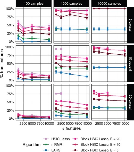
Percentage of true causal features extracted by different feature selectors. Each data point represents the mean over 10 replicates, and the error bars represent the standard error of the mean. Lines are discontinued when the algorithm required more memory than the provided (50 GB). Note that in some conditions mRMR’s line cannot be seen due to the overlap with LARS

We wanted to test these conclusions using a non-linear, real-world dataset. We selected four image-based face recognition tasks (Section 3.3). In this case, we selected different numbers of features (10, 20, 30, 40 and 50). Then, we trained random forest classifiers on these subsets of the features, and compared the accuracy of the different classifiers on a test set (Supplementary Fig. S1). Block HSIC Lasso displayed a performance comparable to vanilla HSIC Lasso, and comparable or superior to the other methods. This is remarkable, since it shows that, in many practical cases, block HSIC Lasso does not need more samples to achieve vanilla HSIC Lasso performance.

4.2 Adjusting by covariates improves feature selection

To evaluate the impact of covariate adjustment, we worked on a synthetic dataset (Section 3.2) with the following experimental parameters: $n=1\hspace{0.17em}000$⁠; $d=\{100,2500,5000,10\hspace{0.17em}000\}$ features; seven causal features. Two covariates were generated by taking two causal features and adding Gaussian noise (mean = 0; standard deviation = 0.5). In the experiment shown in Supplementary Figure S2, we tested the ability of (block) HSIC Lasso to retrieve exclusively the remaining five causal features adjusting for the covariates. We observe that block HSIC Lasso is able to find more relevant features when it adjusts for known covariates.

4.3 Block HSIC Lasso is computationally efficient

In our experiments on synthetic data, vanilla HSIC Lasso runs into memory issues already with 1000 samples (Fig. 1). This experiment shows how block HSIC Lasso keeps the good properties of HSIC Lasso, while extending it to more experimental settings. Block HSIC Lasso with B = 20 reaches the memory limit only at 10 000 samples, which is already sufficient for most common bioinformatics applications. If larger datasets need to be handled, it can be done by using smaller block sizes or a larger computer cluster.

We next quantified the computational efficiency improvement the block HSIC estimator brings. We compared the runtime and the peak memory usage in the highest dimensional setting where all methods could run (⁠$n=1000,\hspace{0.17em}d=2500$⁠, 20 causal features) (Fig. 2). We observe how, as expected, block HSIC Lasso requires an order of magnitude less memory than vanilla HSIC Lasso. Block versions also run notoriously faster, thanks to the lower number of operations and the parallelization. mRMR is 10 times faster than block HSIC Lasso, at the expense of a clearly lower accuracy. However, a fraction of this gap is likely due to mRMR having been implemented in C++, while HSIC Lasso is written in Python. In this regard, there is potential for other faster implementations of (block) HSIC Lasso.

Fig. 2.

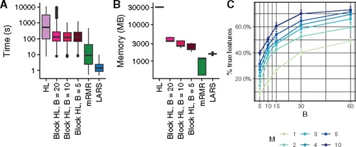
Computational resources used by the different methods. (A) Time elapsed in a multiprocess setting. (B) Memory usage in a single-core setting. (C) Number of correct features retrieved on synthetic data (⁠$n=1000,\hspace{0.17em}d=2500$⁠, 20 causal features) by block HSIC Lasso at different block sizes B and number of permutations M

4.4 Block HSIC Lasso improves with more permutations

We were interested in the trade-off between the block size and the number of permutations, which affect both the computation time and accuracy of the result. We tested the performance of block HSIC Lasso with $B=\{5,10,15,30,60\}$ and $M=\{1,2,3,5\}$ in datasets of $n=1000,\hspace{0.17em}d=2500$ and 20 causal features. As expected, causal feature recovery increases with M and B (Fig. 2C), as the HSIC estimator approaches its true value.

The memory usage $O(\mathit{dnBM})$ of several of the conditions was the same, e.g. B = 10, M = 3 and B = 30, M = 1. Such conditions are indistinct from the points of view of both accuracy, and memory requirements. In practice, we found no major differences in runtime between different combinations of B and M. Hence, a reasonable strategy is to fix B to a given size, and tune the M to the available memory/desired amount of information. This strategy, however, should be adapted to fit properties of the data. More specifically, GWAS data are notably sparse, and as result a small block size would result in many blocks consisting entirely of zeros, which would hence be uninformative. In such cases, it might be interesting to prioritize larger block sizes, and fewer permutations.

4.5 Block HSIC Lasso finds more relevant features

We tested the dimensionality reduction potential of different feature selectors. We selected a variable number of features from different multi-class biological datasets, then used a random forest classifier to retrieve the original classes (Section 3.2). The underlying assumption is that only selected features which are biologically relevant will be useful to classify unseen data. To that end, we evaluated the classification ability of the biomarkers selected in four gene expression microarrays (Fig. 3) and three scRNA-seq experiments (Supplementary Fig. S3). Unsurprisingly, we observe that non-linear feature selectors perform notably better than linear selectors. Of the non-linear methods, in virtually all cases block HSIC Lasso showed similar or superior performance to mRMR. Interestingly, as little as 20 selected genes retain enough information to achieve a plateau accuracy in most experiments.

Fig. 3.

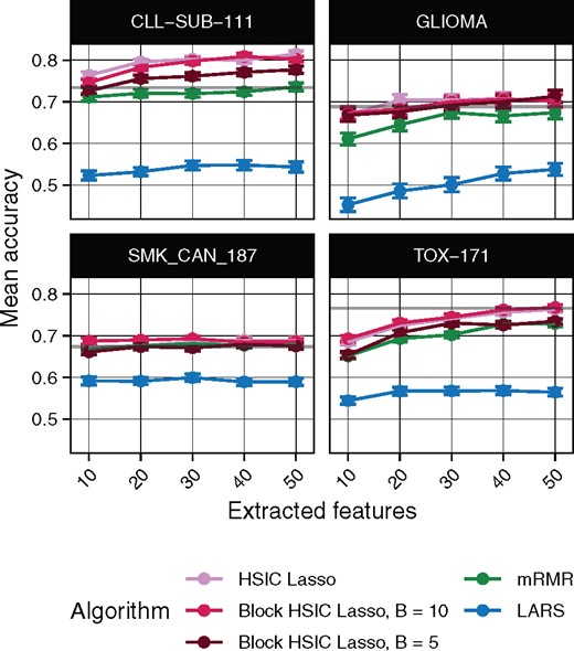
Random forest classification accuracy of microarray gene expression samples after feature extraction by the different methods. The gray line represents the mean accuracy of 10 classifiers trained on all the dataset

Surveying ${10}^5-{10}^6$ SNPs in ${10}^3-{10}^4$ patients, genome-wide association (GWA) datasets are among the most high dimensional in biology, an unbalance which worsens the statistical and computational challenges. We performed the same evaluation on three WTCCC1 phenotypes (Section 3.3). As a baseline, we also computed the accuracy of a classifier trained on all the SNPs (Supplementary Table S1). We observe that a feature selection prior step is not always favorable: LARS worsens the classification accuracy by 5–10%. On top of that, LARS could not select any SNP in 2 out of the 15 experimental settings. On the other hand, non-linear methods improve the classification accuracy by 10%, with mRMR and block HSIC Lasso achieving similar accuracies. In fact, those two selected the same 14 out of 30 SNPs when we selected 10 SNPs in each the three datasets with each method (Supplementary Fig. 5).

4.6 Block HSIC Lasso is robust to ill-conditioned problems

Single-cell RNA-seq datasets differ from microarray datasets in two ways. First, the number of features is larger, equaling the number of genes in the annotation (⁠$>20\hspace{0.17em}\hspace{0.17em}000$⁠). Second, the expression matrices are very sparse, due to biological variability (genes actually not expressed in a particular cell) and dropouts (genes whose expression levels have not been measured, usually because they are low, i.e. technical zeroes). In summary, the problem is severely ill conditioned, and the feature selectors need to deal with this issue. We observed that block HSIC Lasso runs reliably when faced with variations in the data, even on ill-conditioned problems like scRNA-seq. In the different scRNA-seq datasets, LARS was unable to select the requested number of biomarkers in any of the cases, returning always a lower number (Supplementary Fig. S4). mRMR did in all cases. However, the implementation of mRMR that we used crashed while selecting features on the full Villani et al. (2017) dataset.

4.7 Block HSIC Lasso for biomarker discovery

4.7.1 New biomarkers in mouse hippocampus scRNA-seq

To study the potential of block HSIC lasso for biomarker discovery in scRNA-seq data, we focused on the mouse hippocampus dataset from Habib et al. (2016), as a list of $1669$ known biomarkers for the different cell types is also provided by the authors. We requested block HSIC Lasso, mRMR and LARS to select the best 20 genes for classification of 8 cell types (Supplementary Table S2). The cell types were four different hippocampal anatomical subregions (DG, CA1, CA2 and CA3), glial cells, ependymal, GABAergic and unidentified cells.

The overlap between the genes selected by different algorithms was empty. We compared the selected genes to the known biomarkers. Out of the 20 genes selected by mRMR, 14 are known biomarkers, a number that goes down to 0 in the case of block HSIC Lasso (Supplementary Fig. S4A). Hence, these 20 genes, which are sufficient for accurately separating the cell types, are potential novel biomarkers. However, we have no reason to believe that HSIC Lasso generally has a higher tendency to return novel genes than other approaches; we merely emphasize that it suggests alternative, statistically plausible biological hypotheses that can be worth investigating.

We therefore evaluated whether the novel genes found by block HSIC Lasso participate in biological functions known to be different between the cell classes. To obtain the biological processes responsible for the differences between classes, we mapped the known biomarkers to GO Biological process categories using the GO2MSIG database (Powell, 2014). Then we repeated the process using the genes selected by the different feature selectors, and compared the overlap between them. The overlap between the different techniques increases when we consider the biological process instead of specific genes (Supplementary Fig. S4B). Specifically, one biological process term that is shared between mRMR and block HSIC Lasso, ‘Adult behavior’ (associated to Sez6 and Klhl1, respectively), is clearly related to hippocampus function. This reinforces the notion that the selected genes are relevant for the studied phenotypes.

Then we focused on potential biomarkers and biologically interesting molecules among those genes selected by block HSIC Lasso. As it is designed specifically to select non-redundant features, often-used GO enrichment analyses are not meaningful: we expect genes belonging to the same GO annotation to be correlated, and HSIC lasso should not accumulate them. Among the top five genes, two mapped to a biological processes known to be involved: the aforementioned Klhl1 and Pou3f1 (related to Schwann cell development). Klhl1 is a gene expressed in seven of the studied cell types and which has been related to neuron development in the past (He et al., 2006). Pouf1 is a transcription factor which in the past has been linked to myelination, and neurological damage in its absence (Jaegle et al., 1996). The only gene among the top five that was expressed exclusively in one of the clusters is the micro RNA Mir670, expressed exclusively in CA1. According to miRDB (Wong and Wang, 2015), Mir670 top predicted target of its 3’ arm is Pcnt, which is involved in neocortex development.

4.7.2 GWAS without assumptions on genetic architecture

We applied block HSIC Lasso (B = 60, M = 1) to three GWA datasets (Section 3.3). It is typical in GWAS to assume a genetic model before performing statistical testing of associations between SNPs and the phenotype. Two common, well-known models are the additive model—the minor allele in homozygosity has twice the effect as the minor allele in heterozygosity—and the dominant model—any number of copies of the minor allele have a phenotypic outcome. Using non-linear models such as block HSIC Lasso to explore the relationship between SNPs and outcome is attractive since no assumptions are needed on how individual SNPs affect the trait. The only assumption is that the phenotype can be explained by a combination of main effects, as block HSIC Lasso does not account for epistasis. On top of that, by penalizing the selection of redundant features, block HSIC Lasso avoids selecting multiple SNPs in high linkage disequilibrium.

In our experiments, we selected 10 SNPs with block HSIC Lasso for each of the three phenotypes. These are the SNPs that best balance high relatedness to the phenotype and not giving redundant information, be it through linkage disequilibrium or through an underlying shared biological mechanism. We compared these SNPs to those selected by the univariate statistical tests implemented in PLINK 1.9 (Chang et al., 2015). Some of them explicitly account for non-linearity by considering dominant and recessive models of inheritance. The number of SNPs that were positive in at least one test were disparate between the studied phenotypes: all 10 in T1D, 5 in RA, and only 2 in T2D.

Specifically, we compared the genome-wide genotypic P-values to the SNPs selected by block HSIC Lasso (Fig. 4). In T1D, block HSIC Lasso selected SNPs among those with the most extreme p-values. However, not being constrained by a conservative P-value threshold, block HSIC Lasso selects five and eight SNPs in RA and T2D, respectively, with non-Bonferroni significant P-values when they improve classification accuracy Interestingly, one of these SNPs can be physically mapped to PFKM (Keildson et al., 2014), a gene previously identified in genome-wide studies of T2D. The selected SNPs are scattered all across the genome, displaying the lack of redundancy between them. This strategy gives a more representative set of SNPs than other approaches common in bioinformatics, like selecting the smallest 10 P-values.

Fig. 4.

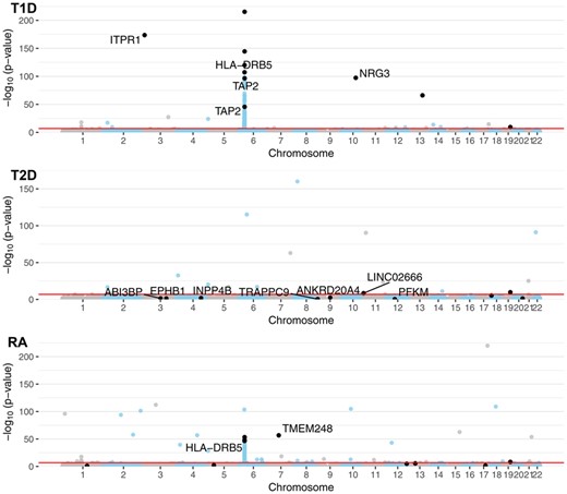
Manhattan plot of the GWA datasets using P-values from the genotypic test. A constant of ${10}^{-220}$ was added to all P-values to allow plotting P-values of 0. SNPs in black are the SNPs selected by block HSIC Lasso (B = 20), 10 per phenotype. When SNPs are located within the boundaries of a gene (±50 kb), the gene name is indicated. The red line represents the Bonferroni threshold with $\alpha =0.05$

5 Discussion

In this work, we presented block HSIC Lasso, a non-linear feature selector. Block HSIC Lasso retains the properties of HSIC Lasso while extending its applicability to larger datasets. Among the attractive properties of block HSIC Lasso we find, first, its ability to handle both linear and non-linear relationships between the variables and the outcome. Second, block HSIC Lasso has a convex formulation, ensuring that a global solution exists, and that it is accessible. Third, the HSIC score can be accurately estimated, as opposed to other measures of non-linearity like mutual information. Fourth, block HSIC Lasso’s memory consumption scales linearly with respect to both the number of features and the number of samples. In addition, block HSIC Lasso can be easily adapted to different problems via different kernel functions that better capture similarities in new datasets. Lastly, block HSIC Lasso can be adjusted for covariates known to affect the outcome, which helps removing confounding effects from the analysis. Due to all these properties, we show how block HSIC Lasso outperforms all other algorithms in the tested conditions.

Block HSIC Lasso can be applied to different kinds of datasets. As other non-linear methods, block HSIC Lasso is particularly useful when we do not want to make strong assumptions about how the causal variables relate to the outcome. Thanks to the advantages mentioned above, HSIC Lasso and block HSIC Lasso tend to outperform other state-of-the-art approaches in terms of both causal features retrieval in simulated data, and classification accuracy on real-world datasets.

Whereas the Lasso is limited to selecting at most as many features as there are available samples (n), for block HSIC Lasso the limitation is nBM. Hence, even if the number of samples is small, block HSIC Lasso can be used to select a larger number of features. If nBM is still limiting, one could replace the ${\ell }_1$ regularization with an elastic-net regularization. However, in most cases, we expect block HSIC Lasso to be used to select a small number of features.

Regarding its potential in bioinformatics, we applied block HSIC Lasso to images, microarrays, single-cell RNA-seq and GWAS. The two latter involve thousands of samples, making it unfeasible to run vanilla HSIC Lasso on a regular server because of its memory requirements. The selected biomarkers are biologically plausible, agree with the outcome of other methods and provide a good classification accuracy when used to train a classifier. Such a ranking is useful, for instance, when selecting SNPs or genes to assay in in vitro experiments.

Block HSIC Lasso’s main drawback is the memory complexity, markedly lower than in vanilla HSIC Lasso but still $O(\mathit{dnB})$⁠. Memory issues might appear in low-memory servers in cases with a large number of samples n, of features d, or both. However, through our work on GWA datasets, the largest type of dataset in bioinformatics, we show that working on these datasets is feasible. Another drawback, which block HSIC Lasso shares with the other non-linear methods, is their black box nature. Block HSIC Lasso looks for biomarkers which, after an unknown, non-linear transformation, would allow a linear separation between the samples. Unfortunately, we cannot access this transformed space and explore it, which makes the results hard to interpret.

Funding

Computational resources and support were provided by RIKEN AIP. H.C-G. was funded by the European Union’s Horizon 2020 research and innovation program under the Marie Skłodowska-Curie [666003]. S.K. was supported by the Academy of Finland (292334, 319264). M.Y. was supported by the JST PRESTO program JPMJPR165A and partly supported by MEXT KAKENHI 16H06299 and the RIKEN engineering network funding.

Conflict of Interest: none declared.