


Abstract
Accurate prediction of loop structures remains challenging. This is especially true for long loops where the large conformational space and limited coverage of experimentally determined structures often leads to low accuracy. Co-evolutionary contact predictors, which provide information about the proximity of pairs of residues, have been used to improve whole-protein models generated through de novo techniques. Here we investigate whether these evolutionary constraints can enhance the prediction of long loop structures.
As a first stage, we assess the accuracy of predicted contacts that involve loop regions. We find that these are less accurate than contacts in general. We also observe that some incorrectly predicted contacts can be identified as they are never satisfied in any of our generated loop conformations. We examined two different strategies for incorporating contacts, and on a test set of long loops (10 residues or more), both approaches improve the accuracy of prediction. For a set of 135 loops, contacts were predicted and hence our methods were applicable in 97 cases. Both strategies result in an increase in the proportion of near-native decoys in the ensemble, leading to more accurate predictions and in some cases improving the root-mean-square deviation of the final model by more than 3 Å.
Supplementary data are available at Bioinformatics online.
1 Introduction
The regions of a protein structure not in α-helices or β-sheets are known as loops and often facilitate function. Loops are typically found on the protein surface (Lins et al., 2003), and therefore are involved in many interactions with other entities, from small molecules to other proteins, and contribute significantly to the overall shape, dynamics and physiochemical properties of the protein (Fiser and Sali, 2003; Papaleo et al., 2016). Prediction of their structures is challenging, due to a reduced level of conservation between homologues compared to the secondary structure elements (Panchenko and Madej, 2005). This means that loop regions are usually the least accurate parts of a homology model (Moult et al., 2018).
A particular obstacle is the prediction of long loop structures. It has been shown that for short loops, the Protein Data Bank (PDB) (Berman et al., 2000) already contains the vast majority of possible conformations (Bonet et al., 2014; Fernandez-Fuentes and Fiser, 2006); as such, it should be possible to model most short loops via knowledge-based approaches. For long loops, the increased number of potential conformations coupled with the lack of structural coverage in the PDB means that this approach will often fail. Ab initio or hybrid methods are therefore required, though this typically leads to lower quality predictions due to difficulties in efficiently exploring the conformational space and correctly selecting near-native models (Marks et al., 2017). Models of long loops are therefore usually less accurate than those of short loops. For example, the average root-mean-square deviation (RMSD) for predictions made by the knowledge-based algorithm LoopIng was 1.01 Å for 6-residue loops and 2.82 Å for 16-residue loops (Messih et al., 2015). For the same set of targets, the ab initio method LEAP achieved accuracies of 0.49 and 4.90 Å for the 6- and 16-residue loops, respectively (Liang et al., 2014). Since 20% of protein loops contain 10 or more residues, and 70% of PDB entries of unique sequence have at least one long loop, it is important that this issue is addressed, and that our ability to model these loops is improved.
The field of de novo (or template-free) structure prediction has benefited from recent advances in the prediction of evolutionary constraints (de Oliveira et al., 2017). Given a multiple sequence alignment, the spatial proximity of residues can be inferred from patterns in their observed mutations. Residue pairs that mutate in a correlated fashion are likely to be structural neighbours, since a pair of interacting residues must vary together to maintain the interaction, and hence conserve protein structure and function. The inferred contacts have then been used as structural constraints, either to guide the conformational search or to filter and rank decoys post-generation (e.g. Braun et al., 2015; de Oliveira et al., 2018; Hopf et al., 2012; Jones et al., 2015; Kamisetty et al., 2013; Kim et al., 2014; Kosciolek and Jones, 2014; Marks et al., 2011, 2012; Ovchinnikov et al., 2015). In this paper we consider whether predicted contacts may also be a viable source of information in a homology modelling setting, e.g. to improve regions of a protein model where the relationship between the target and template is not straightforward.
In this work, we report how predicted contacts can be valuable in the context of modelling long loops (of 10 or more residues). We have explored two protocols with which to do this. The first, for which we use the hybrid loop prediction software Sphinx (Marks et al., 2017), is to filter out conformations from a pre-existing decoy ensemble based on whether they satisfy the set of contacts predicted for the target. The second method involves applying constraints to the decoy generation step to narrow the conformational search space; we demonstrate this approach using the ab initio loop prediction algorithm within MODELLER (Fiser et al., 2000; Fiser and Sali, 2003). In each case we achieve a marked improvement in accuracy—models made by Sphinx are on average 0.53 Å closer to the native structure, while MODELLER’s predictions are improved by an average of 0.49Å. For several targets, improvements of over 3 Å were observed.
2 Materials and methods
2.1 Target set selection
As a training set, we used the set of general loop targets used in Marks et al. (2017). All preliminary investigations into the use of predicted contact information were carried out using this set. The results reported in this paper relate to our test set of long loops (10 residues and above), referred to as the ‘general loop’ target set. These loops were selected as follows. Using PISCES (Wang and Dunbrack, 2003), we extracted a set of protein structures from the PDB with better than 2 Å resolution, a maximum R-value of 0.3, and a maximum sequence identity of 40%. Any PDB entries that were included in or were identical in terms of sequence to the training set were excluded. The loop regions of the remaining proteins were then identified using DSSP (Joosten et al., 2011)—we considered loops to be residues located between helices and strands (DSSP assignments H, G, I and E) of three residues in length or more. Loops with missing atoms or non-standard residue types were ignored. From these we selected a final test set of 135 loops, containing 15 of each length from 10 to 18 residues inclusive, with each target coming from a different PDB entry.
We have also tested our protocols on a set of loops from membrane proteins, specifically those that connect transmembrane segments. Lists of PDB structures relating to membrane proteins were downloaded from three online databases: the Membrane Proteins of Known 3D Structure database (White, 2009), the Protein Data Bank of TransMembrane proteins (Kozma et al., 2013; Tusnàdy et al., 2004) and the Orientations of Proteins in Membranes database (Lomize et al., 2012). The orientation of each structure within the lipid bilayer was predicted using iMembrane (Kelm et al., 2009); only proteins that were predicted to cross the whole membrane layer were retained. We used PISCES to cull this selection of structures based on resolution and sequence identity (maximum sequence identity 60%, maximum resolution 3 Å), resulting in a set of 670 proteins. Loop regions were identified as described above, and the resulting set was further filtered to include only loops that are situated in close proximity to the membrane (within five residues on each side). Our final set of targets contained 160 loops between 10 and 20 residues in length (up to 20 per length, depending on how many were available). Full lists of targets are given in the Supplementary Material, and are labelled with the following notation: PDB code + chain ID_start residue_end residue.
2.2 Contact prediction with MetaPSICOV
Residue–residue contacts were predicted using MetaPSICOV version 1.04 (Jones et al., 2015). MetaPSICOV makes use of a number of other algorithms. PSIPRED (version 4.01) (Jones, 1999) and SOLVPRED are used to predict secondary structure and solvent exposure, respectively; for this we used the ‘uniref90’ database from UniProt (Chen et al., 2017), as recommended by the authors. Multiple sequence alignments were generated by MetaPSICOV using HHblits version 3.0.0 (Remmert et al., 2012) and the ‘uniprot20_2016_02’ database. MetaPSICOV computes its results from a consensus of three other predictors—our implementation used PSICOV version 2.1 (Jones et al., 2012), FreeContact version 1.0.21 (Kajàn et al., 2014) and CCMpred version 1.0.0 (Seemayer et al., 2014). Sequence databases were downloaded in October 2017.
For each protein in the target sets, we extracted the contacts from the MetaPSICOV output (stage 2 results) that involve at least one target loop residue and have a score of over 0.5 (referred to henceforth as ‘loop contacts’). Trivial contacts (those between residues fewer than five residues apart in the protein sequence) are not given by MetaPSICOV and were therefore not considered (these contacts appear not to affect results—see Supplementary Material). In accordance with the definition used to train and test MetaPSICOV (Jones et al., 2015), we considered a contact to be satisfied if the Cβ atoms of the two residues (or Cα for glycine) were <8 Å apart.
If no contacts were predicted for a target, we did not consider it further. Additionally, we found during our preliminary work that for cases with only a single predicted loop contact, the incorporation of this information into the loop modelling protocol either had no significant impact on accuracy (if the predicted contact was correct), or was detrimental (if it was incorrect). Therefore we also excluded targets for which only one loop contact was predicted.
2.3 Loop structure prediction with Sphinx—filtering the decoy ensemble based on predicted contacts
Decoy ensembles were generated using the hybrid loop prediction algorithm Sphinx, as described by Marks et al. (2017). For the prediction of loops in the general target set, we used default parameters, and a database of loop fragments. This contained the loop structures of all PDB entries with non-identical sequences (according to PISCES, using the structure with the best resolution for each sequence), plus three residues on each side, split into all possible fragments of 3–30 residues in length [the same database as previously described in Marks et al. (2017)]. The minimization step used in the original Sphinx paper was omitted to reduce computation time. In all cases, fragments from structures with identical sequences to the target protein were ignored. We produced models in two ways: by using the standard Sphinx implementation, and by integrating the results of contact prediction into the ranking procedure.
The decoys were then ranked by the statistical potential and contact scores separately, after which a consensus ranking was produced by summing the ranks achieved for each decoy by each scoring method. This ranking was used to select the top 500 decoys; these were then scored as normal using SOAP-Loop (Dong et al., 2013; Marks et al., 2017).
When using Sphinx to predict the structures of loops from membrane proteins, we used a specific version of Sphinx (SphinxMembrane), analogous to the antibody H3-specific version of Sphinx described by Marks et al. (2017). In this version, the internal dihedral angle data were calculated from a set of membrane protein loops, the number of fragments Sphinx uses to build decoys is doubled, and the fragment database only consists of membrane protein loop structures. Both the dihedral data and database were generated from the set of loops connecting transmembrane segments described in Section 2.1, however the dihedral distributions were made less sparse using the resampling methodology described by Marks et al. (2017).
2.4 Loop structure prediction in a non-native environment
To investigate the effect of incorporating predicted contacts when modelling loops in a non-exact environment, we generated models for the proteins of the general target set using MODELLER (Sali and Blundell, 1993). Templates were selected using BLAST (Altschul et al., 1990) and the ‘pdbaa’ database; we used the template with the highest BLAST score, excluding structures that have the same sequence as the target. The sequences of the target and template were aligned with Clustal Omega (Sievers et al., 2011). To ensure that the models had at least the correct fold, and the loop anchor residues were approximately in the correct place, models with a template modelling (TM)-score of below 0.5 [as calculated with TM-align (Zhang and Skolnick, 2005)] or an anchor RMSD of over 3 Å were excluded from the study. Anchor residues were defined as two residues on each side of the loop. Sphinx was executed as described in Section 2.3 to remodel the target loops.
2.5 Loop structure prediction with MODELLER—applying constraints to decoy generation
The ab initio loop prediction algorithm within the MODELLER package allows the user to apply constraints during the generation of possible conformations. By using the loop contacts predicted by MetaPSICOV as constraints, exploration of the conformational space should be directed towards more native-like structures, leading to a better quality decoy ensemble and hence more accurate predictions.
To account for the possibility of incorrect contacts, for each decoy generated we selected a random subset of the MetaPSICOV predictions of size 1–N (the total number of contacts), and used these as constraints. Constraints were applied in the form of an ‘upper bound’ function, where distances above a cutoff value have a detrimental effect on the decoy’s score. Consistent with the MetaPSICOV definition we specified a distance cutoff of 8 Å, and we used a σ value of 0.1. As with the Sphinx tests described above, we compared this constrained version to the standard MODELLER algorithm (i.e. no constraints). In each case, we generated 1000 decoys for each target (built onto the crystal structure), used the ‘loopmodel’ class with the ‘slow’ refinement level, and produced a final ranking with the SOAP-Loop scoring function.
2.6 RMSD calculations
All RMSD values for the loop models were obtained after superposition of the model and native structures ignoring the loop region, and were calculated using the coordinates for the backbone atoms of the loop (i.e. N, Cα, C and O). This is a global RMSD (Deane and Blundell, 2001).
3 Results
3.1 Results of contact prediction for loop regions
The contact prediction accuracy achieved by MetaPSICOV for the test set, considering only contacts that involve at least one residue of the target loop, is reported in Table 1. Of the 135 target loops, two or more loop contacts were predicted for 101 (75%—see Supplementary Material for full details). The average number of contacts predicted for a loop was 16.9; the maximum predicted was 84 (for a 16-residue loop). On average, 58.7% of loop contacts were accurate. This is lower than the accuracy achieved for contacts predicted within the rest of the protein (average accuracy =67.2%), potentially reflecting the increased variability in loop sequences compared to regions with more conserved structure. No clear trends were observed across different loop lengths. Most of the predicted contacts (90%) were between one target loop residue and one residue located elsewhere in the protein.
Details of MetaPSICOV predictions for the test set
| Loop length | Number of targets | No. with >1 predicted loop contacts | Average no. of loop contacts | Average accuracy (%) |
|---|---|---|---|---|
| 10 | 15 | 14 | 16.8 | 65.6 |
| 11 | 15 | 13 | 16.2 | 53.5 |
| 12 | 15 | 13 | 15.5 | 59.3 |
| 13 | 15 | 8 | 15.6 | 45.3 |
| 14 | 15 | 11 | 20.3 | 36.4 |
| 15 | 15 | 12 | 11.1 | 62.8 |
| 16 | 15 | 8 | 30.0 | 68.6 |
| 17 | 15 | 12 | 17.8 | 68.2 |
| 18 | 15 | 10 | 12.1 | 65.7 |
| ALL | 135 | 101 | 16.9 | 58.7 |
Note: The numbers refer to predicted contacts where at least one of the residues is part of the target loop. Only targets for which more than one loop contact was predicted are considered. The final row (highlighted in bold text) shows data calculated for the entire target set across all loop lengths.
Other studies have shown that the accuracy of predicted contacts across the entire protein is related to the number of effective sequences (Neff) in the multiple sequence alignment used to infer them (Jones et al., 2015; Ovchinnikov et al., 2015). Using the values for Neff reported by MetaPSICOV, we investigated this relationship for predicted loop contacts, but found no clear relationship between Neff and the accuracy of our predicted loop contacts. The accuracy of prediction is also independent of the presence of gaps in the alignment (see Supplementary Material).
3.2 Sphinx results—filtering the decoy ensemble based on predicted contacts
In this section, we report the results of our investigation into using predicted contacts to filter out inaccurate conformations from the decoy ensemble, by incorporating a ‘contact score’ into the first ranking stage of the Sphinx algorithm (see Section 2.3).
3.2.1 Identification of incorrect contacts
Our strategy of ignoring contacts that are never satisfied in the decoy ensemble (Section 2.3) was highly successful in removing incorrect contacts. Four targets were removed from the study since they only had one predicted contact left after this was carried out. For the remaining 97 loops of the general target set, 105 contacts were ignored across 49 targets—all of these were incorrect predictions, suggesting that this could be a standard strategy for identifying false positives. For our targets, this increased the average accuracy of the contacts from 58.7 to 64.2%.
3.2.2 Relationship between number of contacts satisfied and decoy RMSD
If the predicted contacts are to be useful in loop prediction, decoys satisfying the largest number should tend to be the most accurate, and conversely, those that satisfy the least should be the furthest from the native structure. In Figure 1, we show the relationship between the number of contacts satisfied and decoy RMSD for two example targets. For the loop 4B4HA_526_543, there are seven predicted contacts that are satisfied at least once by decoys in the ensemble. MetaPSICOV predicted one further contact, however this was never satisfied by any decoy and was therefore, as discussed previously, assumed to be incorrect and omitted from the analysis (the actual distance between the relevant atoms in the native structure is 20 Å). Decoys that satisfied more of the predicted loop contacts did indeed tend to have lower RMSDs; the average RMSD of decoys satisfying all seven was 1.50 Å, while those satisfying none had an average RMSD of 11.70 Å (Fig. 1A).
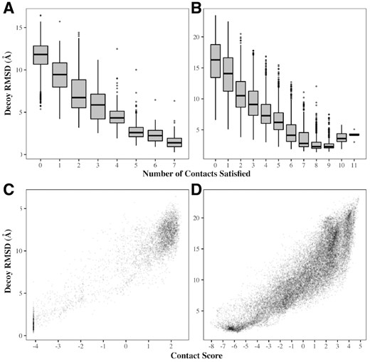
Decoy RMSD versus number of satisfied predicted contacts satisfied (top panels) and contact score (bottom panels) for two examples from the general target set. (A, C) 4BH4A_526_543; an 18-residue loop, with 7 contacts predicted. All of these contacts were correct; the distributions of RMSDs therefore improve as the number of contacts satisfied increases. (B, D) 5CDKA_105_121; a 17-residue loop with 13 predicted contacts, of which 9 were correct. The best distribution of RMSDs is achieved for decoys satisfying nine contacts; decoys which satisfy more than this tend to have higher RMSDs since they are satisfying contacts that are incorrect. In both cases, the contact score correlates with decoy RMSD
A more complicated picture emerges for targets where not all predicted contacts are accurate. For example, MetaPSICOV predicted 13 contacts for the loop 5CDKA_105_121, but only 9 were correct. Therefore, the most accurate decoys were those that satisfied nine contacts (average RMSD =2.73 Å). As shown in Figure 1B, up to this point the distribution of RMSDs improves with increasing numbers of satisfied contacts; beyond this the average decoy accuracy decreases. However, even though some contacts are wrong in the latter case, for both targets the contact score described in Section 2.3 correlates well with RMSD (Fig. 1C and D). Hence, by combining this with Sphinx’s knowledge-based potential, we should be able to select more of the accurate decoys in the ensemble to be in the top 500.
3.2.3 Quality of the decoy ensemble and accuracy of predictions
Figure 2 shows the effect of using contact information on the quality of the top 500 decoys. It shows the change in the number of ‘good’ decoys (RMSD below 2 Å) when using contact information compared to a standard Sphinx run. For the majority of targets (51), filtering the decoy ensemble using predicted contacts increased the number of good conformations. There were only 8 targets out of the set of 97 whose decoy ensembles were made worse. The average accuracy of contact prediction for these 8 targets was 56.5%. For the targets whose decoy ensembles were improved, the average accuracy of contact prediction was higher at 67.2%. In addition, of the eight targets whose results were not improved, seven had predicted contacts where the true Cβ–Cβ distance was over 10 Å.
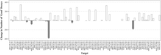
The change in the number of ‘good’ decoys in the top 500 when incorporating predicted contacts into the filtering step, compared to the normal Sphinx protocol. ‘Good’ decoys are defined as those having an RMSD of below 2 Å. The 8 of the 97 targets for which the predicted contacts had a negative effect are indicated with a ‘*’. For the majority of targets, the contact information improved the quality of the decoys in the top 500
The improved quality of the filtered decoy ensemble leads to higher accuracy predictions after the final ranking stage (Table 2). The average RMSD of the best decoy in the filtered set of 500 decreased from 1.76 to 1.55 Å. After ranking with the SOAP-Loop potential, the top-ranked decoy had an RMSD of 3.11 Å, which was 0.60 Å lower than could be achieved without predicted contacts (3.71 Å). The average RMSD of the best decoy in the top 5 was also improved, decreasing from 2.79 to 2.37 Å.
Prediction accuracies achieved by Sphinx on crystal structures, both with (C) and without (−) using contact information
| Target length | No. targets | Best | Best top 500 | Top-ranked | Best top 5 | |||
|---|---|---|---|---|---|---|---|---|
| (−) | (C) | (−) | (C) | (−) | (C) | |||
| 10 | 14 | 0.69 | 0.79 | 0.78 | 2.34 | 1.22 | 2.05 | 1.15 |
| 11 | 13 | 0.84 | 0.97 | 1.24 | 2.05 | 2.55 | 1.66 | 1.77 |
| 12 | 12 | 0.93 | 1.40 | 1.15 | 3.64 | 2.61 | 2.38 | 1.69 |
| 13 | 8 | 0.95 | 1.49 | 1.35 | 3.13 | 2.39 | 2.00 | 1.97 |
| 14 | 9 | 1.49 | 2.19 | 2.01 | 5.23 | 4.21 | 3.56 | 3.22 |
| 15 | 11 | 1.87 | 2.79 | 2.10 | 4.48 | 3.98 | 3.82 | 3.19 |
| 16 | 8 | 1.96 | 2.06 | 2.17 | 4.09 | 4.14 | 3.24 | 3.07 |
| 17 | 12 | 1.16 | 1.78 | 1.60 | 3.51 | 3.51 | 2.85 | 2.43 |
| 18 | 10 | 1.71 | 3.02 | 2.15 | 6.08 | 4.38 | 4.13 | 3.66 |
| ALL | 97 | 1.24 | 1.76 | 1.55 | 3.71 | 3.11 | 2.79 | 2.37 |
Note: Figures reported are backbone RMSDs, averaged across the targets of the relevant length. ‘Best’ refers to the lowest RMSD in the complete decoy ensemble (i.e. before filtering), ‘Best Top 500’ refers to the best decoy in the filtered set of 500, ‘Top Ranked’ is the decoy predicted by SOAP-Loop to be the best and ‘Best Top 5’ refers to the lowest-RMSD decoy in the top 5, again as ranked by SOAP-Loop. Bold values indicate which of the two approaches produced the best result. Predicted contact information improved the accuracy of loop models.
Figure 3 shows a target for which the inclusion of predicted contact information into the ranking scheme produced a significant improvement in accuracy, 2GGSA_111_128 (an 18-residue loop). MetaPSICOV predicted four contacts for this loop; three of these were correct (Fig. 3A). Without using contact information, prediction of this loop’s conformation was challenging and the top 5 decoys (Fig. 3B) were not native-like; the best in this set had an RMSD of 5.35 Å and the top-ranked decoy had an RMSD of 16.17 Å. Conversely, when filtering the decoy ensemble using contacts, the top 5 conformations were all close to the native structure—all had an RMSD of below 2 Å, and the best (which is also the top-ranked) had an RMSD of 1.38 Å. When Sphinx was run normally, i.e. without the contact score, all these five decoys were filtered out at the first ranking stage since they were placed outside the top 500.
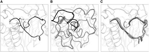
Sphinx predictions for an 18-residue loop target (2GGSA_111_128). Four contacts were predicted for this loop, of which three were correct—panel A shows the native structure with these contacts labelled. When running Sphinx normally, the top 5 decoys (shown in panel B) do not resemble the native structure. The top-ranked decoy has an RMSD of 16.17 Å (coloured black); the best of the top 5 has an RMSD of 5.35 Å. In contrast, by incorporating contact information into the first ranking stage, the top 5 decoys are all native-like, with RMSDs below 2 Å (these decoys are displayed in panel C). The top-ranked decoy in this case, which is also the best in the top 5 (again shown in black), has an RMSD of 1.38 Å
3.2.4 Loop prediction in a non-native environment
It is more common when modelling loops to be refining or filling gaps in a protein model, than predicting missing loops in an experimentally determined structure. Therefore, to achieve a more realistic assessment of the protocols, we ran Sphinx in the same manner, but using protein models as input instead of crystal structures. Since the residues of the protein are not in their native conformations, predicting loop structures in this setting is more challenging. On average, the protein models had a TM-score of 0.94 and an anchor RMSD of 0.77 Å to the native structure (full details are given in the Supplementary Material). Again, we found that the inclusion of predicted contact information improved the accuracy of the resulting loop models (Table 3).
Prediction accuracies achieved by Sphinx, both with (C) and without (−) using contact information, when using model input structures
| Target length | No. targets | Best | Best top 500 | Top-ranked | Best top 5 | |||
|---|---|---|---|---|---|---|---|---|
| (−) | (C) | (−) | (C) | (−) | (C) | |||
| 10 | 12 | 0.91 | 1.12 | 0.99 | 2.54 | 1.98 | 2.07 | 1.51 |
| 11 | 11 | 0.96 | 1.09 | 1.29 | 2.42 | 3.00 | 1.94 | 2.20 |
| 12 | 12 | 1.31 | 2.41 | 1.51 | 4.32 | 3.35 | 2.99 | 2.53 |
| 13 | 8 | 1.13 | 1.63 | 1.58 | 3.29 | 2.74 | 2.81 | 2.20 |
| 14 | 8 | 1.57 | 2.75 | 2.88 | 5.45 | 5.62 | 4.68 | 4.46 |
| 15 | 9 | 1.66 | 2.12 | 1.74 | 5.02 | 4.17 | 3.71 | 2.43 |
| 16 | 4 | 1.66 | 2.06 | 2.00 | 5.04 | 6.31 | 3.94 | 3.68 |
| 17 | 10 | 1.09 | 1.72 | 1.40 | 3.66 | 4.00 | 2.60 | 1.75 |
| 18 | 6 | 0.61 | 1.45 | 0.72 | 5.37 | 0.87 | 3.21 | 0.80 |
| ALL | 80 | 1.19 | 1.78 | 1.52 | 3.91 | 3.40 | 2.96 | 2.31 |
Note: Figures reported are backbone RMSDs, averaged across the targets of the relevant length. ‘Best’ refers to the lowest RMSD in the complete decoy ensemble (i.e. before filtering), ‘Best Top 500’ refers to the best decoy in the filtered set of 500, ‘Top Ranked’ is the decoy predicted by SOAP-Loop to be the best and ‘Best Top 5’ refers to the lowest-RMSD decoy in the top 5, again as ranked by SOAP-Loop. Predicted contact information improved the accuracy of loop models even when the anchors and other surrounding residues are not in their native conformation. Bold values indicate which of the two approaches produced the best result.
As before, omitting contacts that are never satisfied was of benefit; 98 contacts were ignored, of which all but 3 were incorrect. For our targets, this increased the average accuracy of predicted contacts from 58.6 to 63.7%.
3.3 MODELLER results—constraining decoy generation based on predicted contacts
The second strategy we tested for the incorporation of contact prediction into loop modelling was to constrain the generation of decoys such that the resulting conformations are more likely to satisfy the predicted contacts. For this we used MODELLER (see Section 2.5).
Similar to the Sphinx results described above, the incorporation of contact information into the loop modelling protocol improved the accuracy of prediction. Applying constraints based on predicted contacts generally produced decoys that are closer to the native loop conformation than those produced using the standard MODELLER algorithm (see Supplementary Material). On average, the best decoy of the 1000 generated for each target was 0.36 Å closer to the native structure than when using no constraints. This improvement in the quality of the decoy ensemble led to more accurate final predictions. With no contact information, after scoring with SOAP-Loop, the average RMSD of the top-ranked decoy and best of top 5 were 4.75 and 3.28 Å, respectively, whereas these values were 4.26 and 2.76 Å when constraints were applied during decoy generation. Full results are given in the Supplementary Material.
3.4 Modelling membrane protein loops
A group of proteins that are of particular interest, especially in a structure prediction context, are membrane proteins. A large proportion of current drug targets—an estimated 60%—are membrane proteins (Yin and Flynn, 2016), however due to challenges in the experimental determination of their structures there are disproportionately few entries in the PDB. Unfortunately, this lack of structural data also makes modelling difficult, particularly for loop regions due to their variable nature. Any advances made in the prediction of membrane protein structures would therefore aid in narrowing the sequence-structure gap, and would be hugely beneficial in the development of new drugs.
Following the procedure used previously for general protein loops (see Section 2), we predicted residue–residue contacts for a set of loops from membrane proteins using MetaPSICOV. Two or more contacts were predicted for 92 of the 160 targets (58%), with an average accuracy across targets of 65.1% (see Supplementary Material for details). This is higher than the accuracy achieved for the general loop target set. The average number of contacts was lower at 9.5, compared to 16.9.
Omitting contacts that were never satisfied by any decoy was again successful—49 predicted contacts were ignored from 21 targets (2 of these targets were removed from the study at this point as they had one or no contacts remaining). As with the prediction of general loop targets in the native crystal environment, all of these contacts were predicted incorrectly, and therefore removing them from consideration improved the average accuracy of contacts from 65.1 to 68.2%.
Using our membrane protein-specific version of Sphinx, called SphinxMembrane (see Section 2), as well as MODELLER, we investigated whether the extra information offered by contact prediction would improve the accuracy of membrane protein loop prediction, as it did for our general loop set. Results achieved by Sphinx are reported in Table 4 and those of MODELLER are given in the Supplementary Material.
Prediction accuracies achieved by SphinxMembrane, both with (C) and without (−) applying constraints based on predicted contact information, for the membrane protein loop target set
| Target length | No. targets | Best | Best top 500 | Top-ranked | Best top 5 | |||
|---|---|---|---|---|---|---|---|---|
| (−) | (C) | (−) | (C) | (−) | (C) | |||
| 10 | 10 | 0.64 | 0.73 | 1.02 | 2.17 | 2.03 | 2.01 | 1.77 |
| 11 | 10 | 0.97 | 1.75 | 1.62 | 4.50 | 3.25 | 3.17 | 2.38 |
| 12 | 12 | 1.32 | 1.89 | 1.82 | 4.27 | 4.47 | 3.74 | 3.48 |
| 13 | 10 | 1.18 | 1.69 | 1.62 | 3.85 | 4.35 | 2.65 | 2.95 |
| 14 | 6 | 1.05 | 1.48 | 1.62 | 5.33 | 3.19 | 3.40 | 2.35 |
| 15 | 10 | 1.23 | 1.22 | 1.79 | 4.31 | 3.61 | 3.23 | 2.63 |
| 16 | 3 | 1.31 | 3.99 | 1.44 | 9.22 | 4.63 | 7.10 | 3.25 |
| 17 | 8 | 1.20 | 2.19 | 1.57 | 6.65 | 4.56 | 4.19 | 3.76 |
| 18 | 5 | 2.02 | 2.18 | 2.18 | 6.16 | 7.91 | 3.24 | 4.89 |
| 19 | 8 | 1.32 | 1.74 | 1.70 | 3.71 | 2.76 | 1.97 | 1.89 |
| 20 | 8 | 1.17 | 2.92 | 2.76 | 7.80 | 5.84 | 5.54 | 4.80 |
| ALL | 90 | 1.18 | 1.84 | 1.73 | 4.98 | 4.15 | 3.27 | 3.17 |
Note: Figures reported are backbone RMSDs, averaged across the targets of the relevant length. ‘Best’ refers to the lowest RMSD in the complete decoy ensemble (i.e. before filtering), ‘Best Top 500’ refers to the best decoy in the filtered set of 500, ‘Top Ranked’ is the decoy predicted by SOAP-Loop to be the best and ‘Best Top 5’ refers to the lowest-RMSD decoy in the top 5, again as ranked by SOAP-Loop. Predicted contact information enables more accurate predictions to be made. Bold values indicate which of the two approaches produced the best result.
For both algorithms, while accuracies tended to be lower than achieved for the general loop targets, the inclusion of predicted contact information improved results at all stages. Using SphinxMembrane, the best of the top 500, top-ranked and best of the top 5 decoys had average RMSDs of 1.73, 4.15 and 3.17 Å with contacts, respectively, compared to 1.84, 4.98 and 3.27 Å when running the software conventionally.
With MODELLER, we achieved average accuracies of 2.58, 5.35 and 3.88 Å for the best, top and best of top 5 decoys, respectively, when using predicted contacts. Again, this is better than the standard algorithm (which produced values of 2.90, 6.54 and 4.62 Å for the same three measures). This means that we observed an average improvement in accuracy of over an Ångström when considering the top-ranked predictions.
4 Conclusion
The results we report here show that predicted residue–residue contacts, inferred from coevolution, can be used to improve the accuracy of loop structure prediction algorithms. This is true even for typically challenging scenarios, such as modelling in a non-native environment, or the prediction of membrane protein loops.
We have demonstrated that contact prediction can be incorporated in two ways: by scoring and thereby filtering decoys based on whether they satisfy the predicted contacts or not, and by constraining the conformational search step such that the resulting decoys are more likely to satisfy the contacts. Since decoys that satisfy more of the predicted contacts tend to be more native-like, incorporating predicted contacts in these ways leads to improved decoy ensembles and hence better loop models, both in terms of the top-ranked and best of top 5 conformations. It should be possible to apply these concepts to any loop prediction software.
A current limitation is the accuracy of the contact prediction method. On average, we found that contacts predicted for loop regions are less accurate than for more regular secondary structure elements—this means that an appreciable number of the contacts being used to influence the loop prediction procedure are incorrect. Even so, we see an overall improvement after their inclusion, and as methods continue to improve, and more sequences are obtained, it is likely that even better results could be achieved (Ovchinnikov et al., 2017; Wang et al., 2017).
When filtering a pre-generated decoy ensemble, we have found that the accuracy of the contacts being considered can be increased by discarding those that are never satisfied by any decoy in the set. In a non-native environment, 97% of the contacts removed using this approach were incorrectly predicted; when modelling onto the crystal structure we found that all of the ignored contacts were inaccurate.
An advantage of using contact prediction to aid loop modelling is that it allows us to exploit sequence information in addition to structural data. Protein sequences are more numerous than experimental structures, but are normally disregarded when modelling loops. Our methods offer a way of utilizing this relative wealth of information. Moreover, using sequence data may prove to be more beneficial in a homology modelling context than when predicting structures de novo, because more sequences tend to be available for targets for which templates can be found (Kamisetty et al., 2013). Our results show that the incorporation of sequence data is beneficial for challenging situations such as long loop prediction, membrane protein loop prediction and modelling in a non-native environment. Advances could be made for other difficult tasks in the same way, e.g. the prediction of multiple conformations—the set of predicted contacts may reflect the different structures in the ensemble. As the number of sequences continues to increase and algorithms providing structural insights improve, using the variety of information they offer to guide structure prediction will allow us to obtain more accurate and useful protein models.
Acknowledgements
The authors would like to thank Saulo H. P. de Oliveira for his assistance with carrying out contact prediction, and the reviewers for their helpful comments.
Funding
This work was supported by the Engineering and Physical Sciences Research Council [grant reference EP/G037280/1]; and UCB Pharma Ltd.
Conflict of Interest: none declared.
References

