


Abstract
Protein quality assessment (QA) is a crucial element of protein structure prediction, a fundamental and yet open problem in structural bioinformatics. QA aims at ranking predicted protein models to select the best candidates. The assessment can be performed based either on a single model or on a consensus derived from an ensemble of models. The latter strategy can yield very high performance but substantially depends on the pool of available candidate models, which limits its applicability. Hence, single-model QA methods remain an important research target, also because they can assist the sampling of candidate models.
We present a novel single-model QA method called SBROD. The SBROD (Smooth Backbone-Reliant Orientation-Dependent) method uses only the backbone protein conformation, and hence it can be applied to scoring coarse-grained protein models. The proposed method deduces its scoring function from a training set of protein models. The SBROD scoring function is composed of four terms related to different structural features: residue–residue orientations, contacts between backbone atoms, hydrogen bonding and solvent–solute interactions. It is smooth with respect to atomic coordinates and thus is potentially applicable to continuous gradient-based optimization of protein conformations. Furthermore, it can also be used for coarse-grained protein modeling and computational protein design. SBROD proved to achieve similar performance to state-of-the-art single-model QA methods on diverse datasets (CASP11, CASP12 and MOULDER).
The standalone application implemented in C++ and Python is freely available at https://gitlab.inria.fr/grudinin/sbrod and supported on Linux, MacOS and Windows.
Supplementary data are available at Bioinformatics online.
1 Introduction
Proteins play an important role in fundamental biological processes such as biological transport, formation of new molecules, or cellular protection through binding to specific foreign particles such as viruses. This importance has triggered an extensive research of their function and mechanisms involved in these processes. In particular, investigation of protein folding, which plays an essential functional role in living cells, requires costly experiments that can be potentially replaced by cheaper and faster computational methods for modeling undiscovered protein structures (Kmiecik et al., 2016).
A lot of progress has been recently made in protein structure prediction, a computational problem of determining the target protein structure given its amino acid sequence. Most of the methods proposed for protein structure prediction first generate a pool of plausible protein conformations (protein models) and then rank them using a certain QA method to select the top-ranked candidates. Therefore, being aimed at ranking protein models by their quality, QA methods constitute a crucial part of pipelines for protein structure prediction. Usually, these QA methods are based on scoring functions that predict similarity between protein models and the target structures in terms of such similarity measures as RMSD, GDT-TS and TM-score (Zemla, 2003). In particular, RMSD measures the average distance between the atoms of two superimposed protein conformations. GDT-TS and TM-score are designed to assess the quality of protein models being protein size independent and robust to local structural errors (Zemla, 2003).
There are generally two types of QA methods. Consensus-model QA methods decide on the quality of individual protein models based on their statistics in the assessed model pool. In contrast, single-model QA methods consider only atoms of the assessed protein model with no additional information about other models in the pool and hence, these can be used for conformational sampling and structure refinement. Furthermore, the performance of consensus-model QA methods usually depends on single-model QA methods involved in the conformational sampling used for generating pools of assessed protein models. In addition, single-model QA methods are proved to achieve better performance compared to consensus-model QA methods on unbalanced protein model pools and in cases where protein models within assessed pool are very similar (Ray et al., 2012). In addition to these two main types of QA methods, techniques combining both ideas have also been proposed (Jing and Dong, 2017; Maghrabi and McGuffin, 2017), referred to as quasi-single model QA methods.
Among recently proposed single-model QA methods, there are generally two main approaches to design a scoring function: physics-based and knowledge-based (data-driven) approaches (Faraggi and Kloczkowski, 2014; Liu et al., 2014). Physics-based scoring functions are constructed according to some physical knowledge of interactions in the system. This approach takes its roots from the Gibbs free energy minimization principle, which states that all target protein structures minimize the Gibbs free energy over the whole conformational space. However, precise estimation of the Gibbs free energy requires exhaustive sampling of a huge number of conformational states (Cecchini et al., 2009; Tyka et al., 2006), which is computationally intractable in most practical cases. The physics-based approaches are aimed at constructing scoring functions (often called energy potentials or force-fields) that approximate the enthalpic part of the Gibbs free energy and can be estimated efficiently. Usually, these potentials decompose the total energy into a sum of additive terms (contributions) that represent stretching of bonds or angles, dihedral potentials, electrostatic and van der Waals interactions, etc. Alongside with the physics-based approaches, there are so-called knowledge-based approaches that deduce the essential energies of molecular interactions from the structural and sequence databases assuming a certain distribution of conformations or minimizing a certain loss function. The respective scoring functions are typically derived either by machine learning or by estimating the probabilities of certain conformations (statistical QA methods) using statistics of determined native protein structures from structural databases. Supplementary Section A in Supplementary Material overviews several commonly used representative QA methods.
Although plenty of QA methods have been proposed, often they miss such meaningful contributions as solvation-related terms and terms related to hydrogen bonding interactions. However, these contributions are important and generally should be taken into account. For instance, hydrogen bonds provide structural organization of distinct protein folds (Hubbard and Kamran Haider, 2001). In addition, most of QA methods require all-atom protein models as input, and thus their performance critically depends on the accuracy of side-chain packing, that is, positions of the side-chain atoms. These can be modeled with the widely-used SCWRL4 tool (Krivov et al., 2009), as in Cao and Cheng (2016), or any other method (Liang et al., 2011). A possibility of working in a simplified coarse-grained representation of amino acids, as in Kmiecik et al. (2016), overcomes this issue and also reduces the overall computational complexity. Another drawback of many existing protein scoring functions is their discontinuity caused, e.g, by penalties introduced for mismatched inferred and predicted secondary structures. Because of that, these methods cannot be used for gradient-based structure optimization.
In this paper, we propose a novel method for protein quality assessment, the Smooth Backbone-Reliant Orientation-Dependent (SBROD) scoring function. SBROD is a single-model QA method that scores protein models using only geometric structural features along with the explicit representation of solvent generated on a regular grid around assessed proteins. It requires only coordinates of the protein backbone, and thus is insensitive to conformations of the side-chains. In addition, the SBROD scoring function is continuous with respect to coordinates of the protein atoms, which makes it also potentially applicable for being used in molecular mechanics applications.
2 Materials and methods
The workflow of SBROD comprises two stages. First, the method extracts features from each protein model in the dataset. Then, the scoring function assigns a score to each processed protein model based on its features extracted on the first stage. Figure 1 schematically shows the workflow with four groups of geometric features, which are based on the four types of inter-atomic interactions described in detail below. Once these features are extracted and preprocessed, a Ridge Regression model (Draper and Smith, 2014) is trained to predict the GDT-TS of protein models. For the preprocessing, the features are either scaled individually, so that they lie in the range for the whole training set (the Scaler boxes in Fig. 1), or they are normalized, so that the Euclidean norm of each non-zero feature vector is equal to one (the Normalizer boxes in Fig. 1).
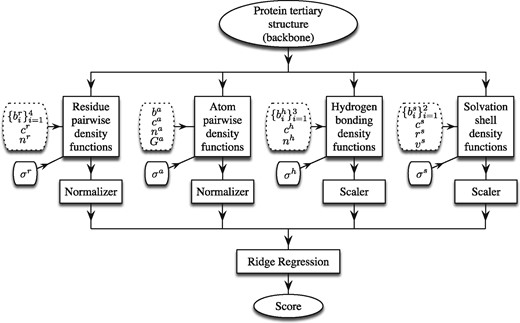
Workflow of the SBROD QA method. The tunable structural parameters are placed in dotted boxes
We should note that we also tested more sophisticated models including Lasso (Tibshirani, 1996), Elastic Net (Zou and Hastie, 2005), Bayesian Regression (Neal, 1996), Ranking SVM (Joachims, 2002) in combination with PCA and Random Projections (Ailon and Chazelle, 2009) for dimensionality reduction, as well as their different modifications and ensembles. However, these did not surpass Ridge Regression significantly regarding the prediction performance. Below, we thoroughly describe the proposed method: from feature generation to training the scoring functions.
2.1 Feature extraction
We build a feature space that reflects four types of physically interpretable interactions: residue–residue pairwise interactions, backbone atom–atom pairwise interactions, hydrogen bonding interactions and solvent–solute interactions. The four respective procedures for feature extraction are implemented in a unified manner. Namely, we iterate over predefined pairs of atomic groups and for each pair we compute feature descriptors that characterize configuration of atoms of one group in the pair with respect to atoms of another group in this pair. The atomic groups are defined by the aforementioned interactions and consist of either individual backbone atoms, atoms that encode orientation of side-chains, atoms specific to the backbone hydrogen bonds, or atoms specific to protein–solvent interactions. We should specifically emphasize that our initial protein model representation contains only heavy backbone atoms. The required positions of backbone amide hydrogens and missing atoms are unambiguously reconstructed using geometry of the input backbone.
Figure 2 schematically shows descriptors that we use. Indices k and l designate a pair of residues in a protein sequence. Symbols and r correspond to distances between atoms, , and denote angles between vector pairs, and is the dihedral angle between two planes passing through carbon atoms and through carbon atoms from residues k and l. In a degenerate case when the dihedral angle is undefined, we choose its value randomly from the interval of possible values. While the intervals of possible values for the angle descriptors are bounded ( and ), the distance descriptors can generally fall into . However, we introduce a cutoff distance and assume interactions between atoms beyond this distance negligible, thereby restricting this interval to the segment .
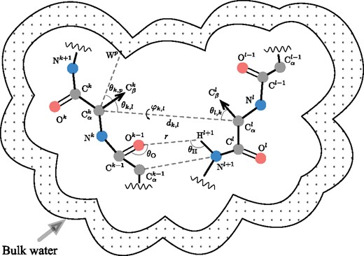
Schematic representation of a protein tertiary structure with four types of structural features. First, the residue–residue pairwise features encode relative geometry of residues k and l. These features are the distance between atoms, and three angular parameters and . Second, each distance between a pair of heavy backbone atoms within a certain cutoff distance, e.g. and , contributes to the backbone atoms’ features. Third, the hydrogen bonding features are based on the orientations of the donor-acceptor pairs of atoms relative to the respective residues, which are defined by the donor angles , the acceptor angles , and the bond lengths r. Finally, the solvation features are comprised of relative positions of the atoms with respect to explicitly generated regular grid of water oxygens (bulk water)
Below we specify four proposed feature extraction procedures, where each is parametrized by tunable parameters shown on the left side of each of the four feature blocks in Figure 1. These parameters change the estimated descriptors and the computation of CNDF.
2.1.1 Residue–residue pairwise features
2.1.2 Backbone atom–atom pairwise features
2.1.3 Hydrogen bonding features
The structural features of the third type represent the hydrogen bonding interactions. To compute CNDF for the hydrogen bonds, we iterate over all donor-acceptor pairs in the backbone within the cutoff distance . To describe the directionality of these interactions, three descriptors shown in Figure 2 are used. These are the distance r between the hydrogen atom H and the oxygen atom O, the donor angle , and the acceptor angle . Then, we compute CNDF with bins as for the case of residue–residue pairwise descriptors. The CNDF accumulates all pairs observed in amino acids that are spaced apart in at least positions in the protein sequence, i.e. we skip all the pairs where the atoms N and O occur in the same residue or residues topologically neighboring in the amino acid sequence.
2.1.4 Solvent–solute features
To take into account the solvent–solute interactions, which make up the fourth type of structural features, we explicitly construct a regular grid of water oxygen atoms around the protein with a period of , as explained in (Artemova et al., 2011; Grudinin et al., 2017). Each point of the grid is located further than from any protein backbone atom but closer than to at least one backbone atom. Note that we use only coordinates of the protein backbone atoms to construct the grid. Then, for each pair of alpha carbon and generated water oxygen atoms within the cutoff distance , we compute two descriptors. These are the distance between these two atoms, and the angle between vectors and pointing towards the side-chain and the water oxygen, respectively. The distance is made somewhat large to implicitly include the interactions of solvent with the protein side-chains.
2.2 Machine learning
2.2.1 Training set
We train the SBROD scoring function on protein models from various CASP (Critical Assessment of protein Structure Prediction) experiments. We used multidomain models, as training on models split into single domains did not provide any noticeable change in the performance of the trained scoring function. For the same reason, we did not filter out any abnormal structures or target structures with all models of poor quality. Server predictions participated in CASP were downloaded from the official CASP website at http://predictioncenter.org/download_area/ and were used in training as protein decoy models.
The total number of structural features extracted from the training protein models was 4 371 840 for the residue–residue features (with 99.92% of zeros on average, i.e. average sparsity), 239 775 for the backbone atom–atom features (96.29% sparsity), 216 for h-bonding (65.32% sparsity) and 138 for solvent–solute (27.32% sparsity). The average total number of nonzero elements in the features was 12 617.
Augmenting training sets with NMA-based decoy protein models. We propose a new approach for augmentation of protein decoy sets. For each target structure in the CASP training set, we generate random structure perturbations based on the Normal Mode Analysis. These decoy models are generated by the NOLB tool (Hoffmann and Grudinin, 2017) combining deformations along 100 slowest normal modes with random amplitudes. We generate 300 decoy models for each target structure with RMSD in the range of .
2.2.2 Model scores
Although there are multiple ways to measure the similarity between protein models and target structures, the most accepted one in the protein structure prediction community is the global distance test total score (GDT-TS). The GDT-TS of a protein model is an average percent of its residues that can be superimposed with the corresponding residues in the target structure under selected distance cutoffs of 1, 2, 4 and . We use the TM-score utility developed by Zhang and Skolnick (2007) to compute the GDT-TS of protein models. The computed GDT-TS of a protein model against its corresponding target structure (see Section 2.2 for notations) is denoted by and treated as the ground truth score of the model .
2.2.3 Ranking model
Optimization. The optimization problem (13) is reduced to a system of linear equations and is solved by the conjugate gradient iterative method implemented in the SciPy Python library (Jones et al., 2001), adapted particularly to sparse matrices of a huge dimension.
Cross-validation. To estimate the best values of the tunable parameters in the feature extraction procedure (, cr, nr, ba, ca, etc., see Fig. 1), and also to select the best regularization parameters α and β in (13) and (14), we use a 3-fold cross-validation on the CASP[5-10] datasets. This is a standard technique for tuning free parameters of a predictive model. More precisely, the original dataset is randomly partitioned into k (here k = 3) even parts. Then, the predictive model is trained on k – 1 parts and validated on the remaining single part. This process is repeated k times with each of the k parts used exactly once as the validation data. The k results from the folds are then averaged to produce a single estimation serving as a criterion of picking the best free parameters of the predictive model. Thus, all the training CASP[5-10] data is used for both training and validation. However, the remaining CASP[11-12] datasets are not involved in this process and are left for the final evaluation. As a result of the described process, the regularization parameters were set to be α = 5, β = 50. The optimal parameters of the feature extraction procedure are specified above in Section 2.1.
3 Results and discussion
We measured the performance of SBROD on the very recent CASP11 and CASP12 Stage1 and Stage2 datasets (Moult et al., 2016). We downloaded these datasets from the official CASP website at http://predictioncenter.org/download_area/ and merged them with the published crystallographic target structures. As a result, we obtained 84 and 83 decoy sets of protein models with the corresponding target structures for the CASP11 Stage1 and Stage2 datasets, respectively. Similarly, we obtained 40 decoy sets for CASP12 Stage1 and 40 decoy sets for CASP12 Stage2. The ground truth GDT-TS values were computed using the TM-score utility (Zhang and Skolnick, 2007). The rest of CASP11 and CASP12 data were filtered out either because their corresponding target protein structures had not been published on the official CASP website or the TM-score utility terminated for those structures with error. No other data were filtered out.
To estimate the performance of a scoring function on a decoy set with a target structure P0 from the test set, we evaluate the predicted scores and then, estimate the following performance measures:
score loss
where is the top-ranked protein model;
the Pearson correlation coefficient between predicted scores and the ground truth for decoy models ;
the Spearman rank correlation coefficient, i.e. the Pearson correlation coefficient between ranks of scores and , where denotes the rank of the value Xj in a set of numbers ;
the Kendall rank correlation coefficient.
Note that the target protein structures P0 are excluded when estimating the performance measures and are used only to compute the ground truth scores of the decoy protein models. Finally, we compute the average of the estimated performance measures over all decoy sets in the test set.
3.1 Smoothness of CNDF
The parameters of calculated CNDF (see Section 2.1 for definition) affect the extracted features and hence the performance of SBROD. Although the parameters of the feature extraction procedures were either optimized on the cross-validation stage or chosen manually, the smoothing parameters σr, σa, σh, σs were tuned independently. Moreover, these parameters were set to zero during all training stages (i.e. only degenerate CNDF with in the truncated Gaussian kernel (1) were used in training) to increase sparsity of the features in training sets, which reduced the complexity and made the training tractable.
To optimize the smoothing parameters and thereby to improve the scoring capacity of SBROD, we first trained a distinct scoring function on the CASP[5-9] datasets without smoothing, i.e. . Then, we measured the dependence of the four performance measures described above (mean score loss, mean Pearson, Spearman and Kendall rank correlation coefficients) on values of the smoothing parameters when testing on the CASP10 dataset (Stage1 and Stage2 combined) with different levels of smoothing by changing the support widths of the truncated Gaussian kernels σa, σr, σh, σs. Figure 3 shows the ratio of the prediction performance with and without the feature smoothing. One can see that the smoothing technique improves the performance of the scoring function. According to all the performance measures, the optimal smoothing parameter appeared to be . Thus, we used this value in all other experiments.
![The performance of SBROD on the CASP10 dataset (Stage1 and Stage2 combined) for different values of the smoothing parameters σa=σr=σh=σs=σ. The SBROD scoring function was trained on the CASP[5-9] datasets using features without smoothing (σ = 0)](https://oup.silverchair-cdn.com/oup/backfile/Content_public/Journal/bioinformatics/35/16/10.1093_bioinformatics_bty1037/4/m_bty1037f3.jpeg?Expires=1716406698&Signature=nqRrOOi7OyA8Y~ddIE8~a-feNwAZ5lL1M4OE8vR8MmCtxgI6rgie~ppL--vM9XNFdW6G5Uehg29Aox~2xfgZLidEaLE0XjjkM0PtpkeqABGScaXjosWAX7R~C3qJHklHGYR9KStKac4pLKyndPKNJeEL4RPdOCllX-I6ee3wOMe4~Ost2MtxNrkphvdMF8ySxvoCTjh2oCHpu~BBOExNu6Oxa9qnBHH7UojgtFIJN5f5qGQXP5UcQNH8EyzSx1qm2HoG9hE1vLHpuQAE1icitBcjuGsLjLwBqVYIzvkU3K6Redtidhe23H2LMurh4YFgkrcw7PcCL8WJP5qTYGatyw__&Key-Pair-Id=APKAIE5G5CRDK6RD3PGA)
The performance of SBROD on the CASP10 dataset (Stage1 and Stage2 combined) for different values of the smoothing parameters . The SBROD scoring function was trained on the CASP[5-9] datasets using features without smoothing (σ = 0)
3.2 Feature contributions
To calculate individual contributions for all the four types of structural features, we set to zero all trained weights wi [see Eq. (14)] corresponding to three out of the four feature groups that are not under consideration [see Eq. (13)] and estimated the performance measures on the CASP11 Stage2 test set. Then, we repeated this procedure for each of the other three feature types. Table 1 lists the results. It can be observed that the features corresponding to residue–residue pairwise interactions contribute to the performance of SBROD the most. However, features representing backbone atom–atom pairwise interactions ensure the best GDT-TS loss performance. We should also note that the protein–solvent interactions alone already give information sufficient to score protein models with a fair enough performance. Weights respective to the hydrogen bonds features provide the poorest predictive ability. This might be the case because the information about the hydrogen bonds is already included in other features and can be inferred from the relative orientation of protein residues, for example. Finally, one can see from Table 1 that usage of all the proposed features provides a significant gain in performance of SBROD compared to the individual contributions.
Contributions of different feature groups to the SBROD performance
| Feature groups | GDT-TS loss | Pearson | Spearman | Kendall |
|---|---|---|---|---|
| All features | 0.057 | 0.441 | 0.426 | 0.298 |
| Residue–residue | 0.078 | 0.380 | 0.365 | 0.253 |
| Backbone atom–atom | 0.069 | 0.344 | 0.327 | 0.224 |
| Solvation shell | 0.107 | 0.267 | 0.271 | 0.189 |
| Hydrogen bonds | 0.112 | 0.142 | 0.126 | 0.089 |
Note: This was measured on the CASP11 Stage2 dataset.
3.3 Amount of training data
An interesting question is whether we can improve the performance of our scoring function by training on more decoy sets or by artificially augmenting the training set. To study this, we conducted a computational experiment where we trained SBROD on different subsets of the CASP[5-10] datasets using both CASP server submissions and NMA-based decoy protein models (see Section 2.2.1). The trained scoring functions were validated on the CASP11 Stage2 dataset. Figure 4 shows the learning curves for estimated performance measures. One can observe that the performance of SBROD trained on the NMA-based decoy protein models becomes stable when the number of decoy sets used for training reaches 300, and no further extension of the training set improves this performance. In contrast, the performance of SBROD trained on the CASP protein models grows steadily when increasing size of the training set. Note that usage of both datasets combined together improves the correlation criteria for training sets with more than 150 decoy sets. Finally, Figure 4 makes reasonable the assumption that the performance of SBROD can be improved by extending the training set, e.g. by including the CASP12 protein models.
![Learning curves for the performance of SBROD on the validation set as a function of the number of training decoy sets. The training was performed on random subsamples of CASP[5-10]. The validation was done using the CASP11 Stage2 set](https://oup.silverchair-cdn.com/oup/backfile/Content_public/Journal/bioinformatics/35/16/10.1093_bioinformatics_bty1037/4/m_bty1037f4.jpeg?Expires=1716406698&Signature=FPFRAFPFAOEb35fqo3yEFS1Ij8raeLO-WKZ6tdRA~C5IEyguWe2Pl2LHYyDqIYZubDIypgmEQ~Yu87GG6aVIIsXE5h0JjQeeBGNDerJidCA44RZOvrG8yD6oYcoLVZEAeJ1FbUId~krPmy90teshipYXbnlwnyc5eHkjDMWE-XaleVk3iDuwxM2RpCXi-H3b2qsYmZ2hhXIXCuntNn-JvkgvMvOyPrkk20OqbZEtMpzIR4BHNzdQmbRO8qrJFCfW1I7DAwx9fxaJHr~RZAOfNmpTMhDsJgSnOTXiwvk8AKR9qUXZGwsXdpy7gAnpMuatEEJsuBql9KUD-4rH1Ukh1A__&Key-Pair-Id=APKAIE5G5CRDK6RD3PGA)
Learning curves for the performance of SBROD on the validation set as a function of the number of training decoy sets. The training was performed on random subsamples of CASP[5-10]. The validation was done using the CASP11 Stage2 set
3.4 Comparison with the state-of-the-art
To compare the performance of SBROD against nine state-of-the-art QA methods, we first used the results obtained by Cao and Cheng (2016). They assessed the performance of several QA methods against the ground truth GDT-TS computed with the LGA utility (Zemla, 2003) for structures with side-chains repacked with SCWRL4 (Krivov et al., 2009) on the CASP11 Stage1 and Stage2 datasets. Since the LGA utility (Zemla, 2003) is not openly available, we used the TM-score utility (Zhang and Skolnick, 2007) instead. Nonetheless, SBROD is not sensitive to the side-chains packing, and the difference between the GDT-TS computed by the TM-score and LGA utilities is negligible. Therefore, the measurements estimated by Cao and Cheng (2016) are consistent with ours, measured as described above, and all of these can be fairly compared to each other.
Supplementary Table S1a and b in Supplementary Material list the performance measures computed for the SBROD scoring function (trained on the CASP[5-10] data augmented with the generated NMA-based decoy models, with the CNDF smoothing parameters of on the testing stage) and for nine other state-of-the-art methods on the CASP11 Stage1 and Stage2 datasets, correspondingly. It can be seen that our method outperforms all other methods on both stages of the CASP11 experiment if assessed by the mean score loss, and it is highly competitive to the other methods if assessed by the other performance measures.
We also repeated a similar experiment using the CASP12 Stage1 and Stage2 data. For this experiment, the SBROD function was trained on CASP[5-11] data augmented with the generated NMA-based decoy models, and more recent methods were added for the comparison (Section B in Supplementary Material provides details on those). Table 2 list the results on the original CASP12 server submissions, and Table 3 list the results for the CASP12 data preprocessed with side-chains repacking. As in the previous experiment, we can see that SBROD is highly competitive to the other methods, especially on the Stage2 data.
Performance of the selected QA methods measured on the CASP12 dataset, sorted by the Spearman correlation
| QA Method | Loss | Pearson | Spearman | Kendall | Z-score |
|---|---|---|---|---|---|
| (a) CASP12 Stage1 | |||||
| ProQ2-refine | 0.098 | 0.623 | 0.651 | 0.503 | 2.403 |
| ProQ2 | 0.099 | 0.633 | 0.646 | 0.495 | 2.327 |
| ProQ3-repack | 0.078 | 0.634 | 0.638 | 0.487 | 2.512 |
| ProQ3 | 0.028 | 0.661 | 0.630 | 0.475 | 3.000 |
| SBROD (this study) | 0.076 | 0.649 | 0.612 | 0.462 | 2.535 |
| VoroMQA | 0.085 | 0.611 | 0.554 | 0.414 | 2.460 |
| RWplus | 0.132 | 0.479 | 0.465 | 0.344 | 2.090 |
| (b) CASP12 Stage2 | |||||
| SBROD (this study) | 0.069 | 0.614 | 0.559 | 0.406 | 1.024 |
| ProQ2-refine | 0.096 | 0.590 | 0.538 | 0.388 | 0.731 |
| ProQ3 | 0.089 | 0.572 | 0.535 | 0.386 | 0.898 |
| ProQ2 | 0.091 | 0.578 | 0.529 | 0.381 | 0.809 |
| ProQ3-repack | 0.070 | 0.601 | 0.526 | 0.381 | 1.078 |
| VoroMQA | 0.106 | 0.559 | 0.501 | 0.362 | 0.692 |
| RWplus | 0.103 | 0.417 | 0.378 | 0.265 | 0.778 |
Note: Native protein structures were filtered out from the dataset. The second column lists GDT-TD losses, the last column lists average Z-scores estimated over the dataset.
Performance of the selected QA methods measured on the CASP12 dataset with side-chain repacking by scwrl4 (Krivov et al., 2009)
| QA Method | Loss | Pearson | Spearman | Kendall | Z-score |
|---|---|---|---|---|---|
| (a) CASP12 Stage1 | |||||
| ProQ2-refine | 0.097 | 0.623 | 0.653 | 0.501 | 2.429 |
| ProQ2 | 0.098 | 0.623 | 0.650 | 0.500 | 2.397 |
| ProQ3-repack | 0.095 | 0.630 | 0.640 | 0.490 | 2.223 |
| ProQ3 | 0.060 | 0.631 | 0.617 | 0.470 | 2.581 |
| SBROD (this study) | 0.076 | 0.649 | 0.613 | 0.463 | 2.535 |
| VoroMQA | 0.081 | 0.602 | 0.546 | 0.409 | 2.515 |
| RWplus | 0.124 | 0.481 | 0.464 | 0.341 | 2.102 |
| (b) CASP12 Stage2 | |||||
| SBROD (this study) | 0.069 | 0.614 | 0.559 | 0.406 | 1.024 |
| ProQ2 | 0.086 | 0.594 | 0.540 | 0.393 | 0.881 |
| ProQ3 | 0.082 | 0.614 | 0.539 | 0.392 | 1.026 |
| ProQ2-refine | 0.083 | 0.591 | 0.538 | 0.390 | 0.861 |
| ProQ3-repack | 0.060 | 0.599 | 0.522 | 0.378 | 1.177 |
| VoroMQA | 0.100 | 0.574 | 0.504 | 0.366 | 0.924 |
| RWplus | 0.104 | 0.477 | 0.412 | 0.291 | 0.679 |
Note: Native protein structures were filtered out from the dataset. The second column lists GDT-TD losses, the last column lists average Z-scores estimated over the dataset.
Finally, we assessed the performance of SBROD together with several other QA methods on the MOULDER dataset (Eramian et al., 2006). This is a conventional dataset for testing physics-based and statistical energy potentials. Supplementary Table S2a in Supplementary Material lists the results and one can see that SBROD is among the best performers there as well.
4 Conclusion
In this paper, we presented SBROD, a novel method for the single-model protein quality assessment. SBROD was developed in a general supervised machine learning framework. First, features were extracted and then, a predictive model was trained to construct the SBROD scoring function. It utilizes only geometric structural features, which can be directly extracted from the conformation of the protein backbone. Thus, conformations of the protein side-chains are not taken into account when ranking the protein structures. The SBROD scoring function includes four contributions from residue–residue, backbone atom–atom, hydrogen bonding, and solvent–solute pairwise interactions. Performed computational experiments on diverse structural datasets proved SBROD to achieve the state-of-the-art performance of single-model protein quality assessment. More precisely, on both Stage1 and Stage2 datasets from the CASP11 protein structure prediction exercise (see Supplementary Table S1a and b), SBROD outperformed all other assessed scoring functions if ranked by mean GDT-TS loss, and it provided very competitive correlations with the ground truth GDT-TS values. On the CASP12 dataset (see Tables 2–3) the results of SBROD were also very competitive to the state-of-the-art methods, especially for the Stage2 subsets. It is also worth mentioning that SBROD, being based on the geometrical features only, surpasses many meta algorithms that use as features scores and predictions from other QA methods and tools. At the same time, SBROD is one of the least demanding QA methods and hence it can be also easily used by meta algorithms as a base predictor. The investigated learning curves, which measure the dependence of the SBROD’s performance on the size of the training set, suggest that the method can be significantly improved just by increasing the size of the training set. Furthermore, we proposed a method for augmenting the protein training decoy sets required by supervised learning with the NMA-based decoy protein models. These decoy models can be easily generated by the NOLB tool, which is computationally fast and easy to use, as perturbations of the target protein structures from the training set. The conducted computational experiment revealed that extending the initial training set with the NMA-based perturbations reliably enhances the performance of the learned scoring function if sufficient number of the training data is used. The proposed technique for extracting geometrical features as continuous functions of atomic coordinates makes the SBROD scoring function also continuous in these coordinates. Therefore, it allows to apply SBROD for continuous gradient-based optimization of protein conformations. In addition, since SBROD provides a residue-pairwise-decomposable scoring function for assessment of coarse-grained protein models, it can be also used to assess the backbone conformations for various protein sequences in the computational protein design. The method is freely available at https://gitlab.inria.fr/grudinin/sbrod as a server or as a standalone executable with described use-cases, manuals and scripts used for training and easily adaptable for using with custom datasets. The procedures for feature extraction implemented in C++11 are available on request.
Acknowledgements
The authors thank Research Center for Molecular Mechanisms of Aging and Age-Related Diseases, Moscow Institute of Physics and Technology. The authors also thank Prof. Yury Maximov from Skolkovo Institute of Science and Technology for his valuable advice and Prof. Vadim Strijov from Moscow Institute of Physics and Technology for helpful discussions. The authors also thank Georgy Derevyanko for his valuable help with running ProQ2 and ProQ3 on the CASP12 datasets and Elodie Laine for help with the manuscript.
Funding
This work was partially supported by the Inria Internships Program, L’Agence Nationale de la Recherche (grant number ANR-15-CE11-0029-03) and by the Ministry of Education and Science of the Russian Federation (grant number RFMEFI58715X0011).
Conflict of Interest: none declared.
References

