multiHiCcompare: joint normalization and comparative analysis of complex Hi-C experiments

Abstract

Motivation

With the development of chromatin conformation capture technology and its high-throughput derivative Hi-C sequencing, studies of the three-dimensional interactome of the genome that involve multiple Hi-C datasets are becoming available. To account for the technology-driven biases unique to each dataset, there is a distinct need for methods to jointly normalize multiple Hi-C datasets. Previous attempts at removing biases from Hi-C data have made use of techniques which normalize individual Hi-C datasets, or, at best, jointly normalize two datasets.

Results

Here, we present multiHiCcompare, a cyclic loess regression-based joint normalization technique for removing biases across multiple Hi-C datasets. In contrast to other normalization techniques, it properly handles the Hi-C-specific decay of chromatin interaction frequencies with the increasing distance between interacting regions. multiHiCcompare uses the general linear model framework for comparative analysis of multiple Hi-C datasets, adapted for the Hi-C-specific decay of chromatin interaction frequencies. multiHiCcompare outperforms other methods when detecting a priori known chromatin interaction differences from jointly normalized datasets. Applied to the analysis of auxin-treated versus untreated experiments, and CTCF depletion experiments, multiHiCcompare was able to recover the expected epigenetic and gene expression signatures of loss of chromatin interactions and reveal novel insights.

Availability and implementation

multiHiCcompare is freely available on GitHub and as a Bioconductor R package https://bioconductor.org/packages/multiHiCcompare.

Supplementary information

Supplementary data are available at Bioinformatics online.

1 Introduction

The advent of chromatin conformation capture (3C) technology allowed for the first insights into the three-dimensional (3D) interactome of the genome (Dekker et al., 2002). Following 3C, 4C and 5C, a high-throughput technology, Hi-C, was introduced as a means for the capture of all versus all interactions across the entire genome (Lieberman-Aiden et al., 2009). The structure and interactions of the DNA in 3D space inside the nucleus have been shown to shape the gene expression of cells and define cellular identity (Dowen et al., 2014; Ji et al., 2016; Phillips-Cremins and Corces, 2013; Rao et al., 2014; Vietri Rudan et al., 2015) and in the regulation of tumor suppressors and oncogenes (Hnisz et al., 2016; Rickman et al., 2012; Taberlay et al., 2016; Valton and Dekker, 2016). The dynamic nature of the 3D structure of the genome prompted significant attention to the comparative analysis of multiple Hi-C datasets (Bonev et al., 2017; Dixon et al., 2015).

Soon after Hi-C data became available, it became clear that the data contained biases which affected the construction and analysis of chromatin contact maps (Yaffe and Tanay, 2011). These biases fall into two categories: DNA sequence-driven and sequencing technology-driven. The sequence-driven biases that can be explicitly modeled include GC content, chromatin accessibility, nucleosome occupancy, repetitive elements and other properties of the DNA sequence (O’Sullivan et al., 2013; Yaffe and Tanay, 2011), and are consistent across datasets. The much less understood and hard-to-model technology-driven biases include cross-linking preferences, the choice of restriction enzymes (e.g. HindIII, MboI, DpnII), biotin labeling, chromatin fragmentation and sequencing depth, among others. These biases affect Hi-C datasets unpredictably, justifying the need for joint normalization of multiple datasets. Early studies tended to focus on normalizing individual Hi-C datasets (Imakaev et al., 2012; Knight and Ruiz, 2012; Lieberman-Aiden et al., 2009; Yaffe and Tanay, 2011). These individual methods improve reproducibility of replicated datasets (Hu et al., 2012; Imakaev et al., 2012; Yaffe and Tanay, 2011). However, these methods leave the problem of different biases between multiple Hi-C datasets unaddressed.

Early methods for normalizing and comparing Hi-C datasets were developed to normalize individual datasets and overlap them. The most notable example is the HiCCUPS algorithm (Rao et al., 2014), which detects chromatin interaction ‘hotspots’ in individually normalized Hi-C datasets. Hotspots, i.e. chromatin interactions enriched relative to the local background, are then compared between datasets by simply overlapping them. This approach does not distinguish hotspots detected due to local biases and does not quantify the significance of the differences. Several papers utilized individually normalized Hi-C datasets and overlap-based methods to reveal important insights into the dynamics of the 3D structure of the genome (Bonev et al., 2017; Dixon et al., 2015). However, the overlap-based methods are severely limited in detecting statistically significant chromatin interaction changes.

To the best of our knowledge, only four methods approach a statistically grounded comparison of Hi-C datasets. The diffHic method is an extension of a negative binomial distribution-based analysis operating on count data (Lun and Smyth, 2015). As such, it leaves a user with challenges of sequencing data storage, the computational burden of processing, normalization, summarization and other bioinformatics heavy lifting of Hi-C data. The HOMER method uses a binomial model to compare individually normalized Hi-C datasets (Heinz et al., 2010). The ChromoR method (Shavit and Lio’, 2014) uses a Poisson model to compare Hi-C datasets. The latest method, FIND, exploits a spatial Poisson process to consider spatial dependency between chromatin regions when detecting differentially interacting loci (Djekidel et al., 2018). However, in our tests, these methods failed to detect consistent differential chromatin interactions. Furthermore, all but diffHic methods use individually normalized Hi-C datasets, leaving the technology-driven biases unaccounted for. Thus, the problem of normalization and statistical comparison of multiple Hi-C datasets remains unsolved.

Our method, HiCcompare (Stansfield et al., 2018), was one of the pioneering normalization methods to consider between dataset biases; however, it is limited to only joint normalization and comparison of two datasets. As sequencing costs continue to decrease and availability of Hi-C sequencing data increases, this method will fall short for Hi-C experiments involving comparison of multiple datasets.

We present a method, multiHiCcompare, for joint normalization and comparison of multiple Hi-C datasets. Our method is based on a distance-centric view of Hi-C data, accounting for the fact that chromatin interaction frequencies (IFs) decay with the increasing distance between interacting regions. Our method utilizes cyclic loess regression-based normalization to jointly normalize Hi-C datasets between replicates and conditions. We then present a differential chromatin interaction analysis framework based on a general linear model (GLM)-based approach (McCarthy et al., 2012; Robinson et al., 2010). Our framework operates on interaction counts subset in a distance-centric manner to produce RNA-seq-count-like matrices that can be directly analyzed using the GLM approach. As an output, genomic coordinates of differentially interacting regions are reported in text format, and the results are compatible with Juicer (Durand et al., 2016) for easy visualization. This method, implemented in the multiHiCcompare R package, represents a streamlined and well-documented pipeline for the joint normalization and comparative analysis of multiple Hi-C experiments.

2 Materials and methods

Hi-C data format. multiHiCcompare works on processed Hi-C data in the form of sparse upper triangular matrices, in plain text format. A typical sparse Hi-C matrix is stored in a separate file for each chromosome and contains three columns—the start location for the first interacting regions, the start location for the second interacting region, and the IF for that interaction. When importing data to use in multiHiCcompare, an additional column needs to be added indicating the chromosome number, as the first column. The original HiCcompare package provides functions for converting between full and sparse matrices (Stansfield et al., 2018).

Filtering. Pairs of chromatin regions showing zero IF across all samples are not considered in all analyses. Additional filtering options include filtering out interacting pairs of regions with the average IF below a pre-defined threshold and/or the proportion of zero IF values larger than a pre-defined threshold across multiple datasets. Filtering helps to increase the computational speed when normalizing and comparing the data. Additionally, it removes interactions with low variability and high numbers of zero IFs that may create problems when estimating the parameters of the negative binomial distribution in the comparative analysis step (Lun and Smyth, 2017). Furthermore, filtering helps to increase power by reducing the effect of the multiple testing correction. By default, interaction pairs with an average IF <5 and the proportion of zero IFs larger than 80% are filtered out.

Cyclic loess normalization. We previously developed a loess regression-based method for normalizing two Hi-C datasets (Stansfield et al., 2018). Briefly, the method is based on representing the data on a mean-difference (MD) plot. The MD plot is similar to the MA plot (Bland–Altman plot) (Dudoit et al., 2002) which is commonly used for the visualization of gene expression differences. $M$ is defined as the log difference between the two datasets $M=\mathrm{lo}{\mathrm{g}}_2(\mathrm{I}{\mathrm{F}}_2/\mathrm{I}{\mathrm{F}}_1)$⁠, where $\mathrm{I}{\mathrm{F}}_1$ and $\mathrm{I}{\mathrm{F}}_2$ are IFs of the first and the second Hi-C datasets, respectively. $D$ is defined as the distance between two interacting regions, expressed in unit-length of the resolution of the Hi-C data. A loess regression curve is fit through the MD plot and used to remove global biases by centering the $M$ differences around $M=0$ baseline (Stansfield et al., 2018). In our previous work, we show that joint loess normalization on the MD plot is superior to other common Hi-C normalization methods (ICE, KR, MA) for the purpose of comparison between experimental conditions (Stansfield et al., 2018). We also performed an additional comparison of cyclic loess with HiCNorm (Hu et al., 2012) (Supplementary Fig. S1). The details of cyclic loess are reported in the Supplementary Methods.

Additionally, we implemented a modified version of the fast linear loess (‘fastlo’) method (Ballman et al., 2004) that is adapted to Hi-C data on a per-distance basis. To perform ‘fastlo’ on Hi-C data we first split the data into p pooled matrices. ‘Progressive pooling’ is used to split up the Hi-C matrix by unit distance such that distance 0 is its own pool, distances 1 and 2 are pooled, distances 3, 4, 5 are pooled and so on until all unit distances belong to one of p pools. p is calculated as follows $p=\mathit{ceiling}\left\{\frac{\sqrt{8n_{\mathrm{d}}+1}-1}{2}\right\}\mathrm{ }$where $n_{\mathrm{d}\mathrm{ }}$is the number of unit distances. The solution for the number of pools follows from the quadratic formula solution for triangular numbers. Progressive pooling is required for the fastlo and difference detection steps because each off-diagonal trace of the matrix gets progressively smaller than the last. Thus, progressive pooling allows for normalization and analysis to be performed in a distance-centric manner while maintaining a similar number of contacts in each pool. These pooled contacts are assembled into matrices of IFs. Each matrix will have an $\mathrm{I}{\mathrm{F}}_{\mathit{gj}}\mathrm{ }$value with g interacting pairs for each of the j samples. These p matrices can then be input into the ‘fastlo’ algorithm using the following steps:

1. Create the vector ${\widehat{\mathrm{IF}}}_{\mathit{pgj}}$⁠, the row means of the $p^{\mathit{th}}$ matrix. This is the equivalent of creating an average IF at distance pool $p$⁠.

2. Plot ${\widehat{\mathit{IF}}}_p$ versus $(I{F}_{\mathit{pg}}-\widehat{I{F}_p})$ for each sample $j$⁠. This is equivalent to an MA plot at a genomic distance pool $p$⁠.

3. Fit a loess curve $f\left(x\right)$ to the plot.

4. Subtract $f\left(x\right)$ from sample $j$⁠.

5. Repeat for all remaining replicates.

6. Repeat until the algorithm converges.

The above steps are performed on the log2-transformed IFs. If a parallelization option is specified, the ‘fastlo’ algorithm is parallelized by splitting up the p matrices and sending them to multiple processors. Similar to cyclic loess, fastlo typically converges within two iterations, which is defined as the point when the row means no longer change (Ballman et al., 2004). Additionally, fastlo has been shown to provide similar normalized values as quantile normalization while being almost as fast computationally (Ballman et al., 2004). Both the cyclic loess and fastlo methods are included in the multiHiCcompare package.

After joint normalization, any negative IFs are automatically set to values of 0. All IFs that started with a zero value are reverted to zero after normalization is complete. This is because we are unable to determine if zeros in Hi-C matrices represent a missing value or an actual absence of contact between the pair of regions.

Detection of chromatin interaction differences. After normalization of the data, we can then proceed to the differential analysis. The primary goal of the differential analysis is to detect the maximal number of true differences while minimizing false positives. Approaches that utilize information across replicate high-throughput data (microarrays, RNA-seq, ChIP-seq) have been shown to improve the power of differential analysis (Phipson et al., 2016; Sartor et al., 2006; Smyth, 2004; Yu et al., 2011). Adopting the distance-centric view of Hi-C data (the off-diagonal vectors in chromatin interaction matrices, Fig. 1), a comparison with other sequencing technologies can be drawn. Similar to RNA-seq read counts, Hi-C IFs may have differing amounts of biological variation across replicates.

Fig. 1.

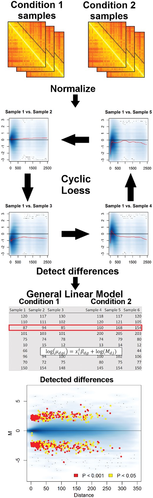
Flowchart for a multiHiCcompare analysis. Pre-processed Hi-C data are read in and then normalized using the cyclic loess (or fastlo) methods. Then ‘progressive pooling’ of the off-diagonal (distance-centric) IFs into a matrix format is performed for input into either an exact test or GLM. Finally, the results of the comparison are shown on a composite MD plot indicating where the differences occurred

As Hi-C reads forming pairwise IFs are count based, the IFs can be modeled using a negative binomial distribution (Robinson and Smyth, 2007) (Supplementary Fig. S2). The distributions of distance-centric vectors of interaction counts can be approximated by the NB distribution, and this approximation holds at different resolutions of Hi-C data and different distances between interacting regions. Thus, the GLM framework of differential gene expression analysis developed for RNA-seq (Anders and Huber, 2010; Auer and Doerge, 2010; Baggerly et al., 2003, 2004; Hansen et al., 2011; Lu et al., 2005; McCarthy et al., 2012; Robinson et al., 2010; Robinson and Smyth, 2007, 2008) can be adapted for differential analysis of IFs. We adapted this framework to process IFs represented as p ‘progressively pooled’ distance-centric matrices with g rows (indices for interacting pairs of regions) and i columns (indices for replicates, Fig. 1). The ‘progressive pooling’ strategy is aimed to increase the robustness of statistical estimates across the whole range of distances between interacting regions. Its adaptation for the GLM framework is described in Supplementary Methods.

Benchmarking multiHiCcompare. To accurately benchmark a method, data with ground truth differences are required (Dozmorov et al., 2010). As there is no gold standard for differential interactions in Hi-C data, we used technical replicates from HCT-116 colorectal cancer cell line at 100 KB resolution for chromosome 22 (Rao et al., 2017) to generate a set of 4×4 Hi-C matrices with ground truth differences. To create this dataset, we used four technical replicates (‘Normal; Biological Sample 2’) (Supplementary Table S1) and created an additional four Hi-C datasets by adding random noise to each of them. Noise was estimated by fitting the distributions of the differences between the replicate dataset’s IFs. The differences were found to follow a roughly normal distribution with means near 0 and SDs between 8 and 11. Thus, to add noise to our ‘simulated’ replicates we sampled from a normal distribution with mean 0 and SD of 10. The noise matrix was then added to the real Hi-C data to produce the simulated replicates. This created a total of eight semi-simulated replicate datasets, suitable for the 4×4 group comparison.

Table 1.

Differential interaction statistics from multiHiCcompare and diffHic for chromatin interaction differences experimentally validated by FISH

	multiHiCcompare				diffHic
Interaction	logFC	logCPM	P-value	FDR	logFC	logCPM	P-values	FDR
FYN - MOXD1	−2.113	10.093	<0.001	0.007	0.733	1.134	0.002	0.042
HEY2 - MOXD1	1.232	11.182	<0.001	<0.001	0.67	2.625	<0.001	0.002
SERPINB9 - MOXD1	−2.227	9.621	0.008	0.356	−1.27	−0.151	0.001	0.016
FYN - HEY2	−2.113	10.093	<0.001	0.007	−1.545	0.621	<0.001	<0.001

Note: ‘Interaction’—the genes interacting identified by FISH, ‘logFC’—the log2 fold change of IF difference between conditions, ‘logCPM’—the between-conditions average log counts per million of the IFs, for multiHiCcompare and diffHic results, respectively.

A pre-specified number of ground truth differences were added in randomly to the chromatin interaction matrices. The randomly selected interacting pairs had their IFs set to the mean of all samples and then Gaussian noise sampled from a N(0,σ) distribution was added to the IFs. σ is defined by fitting a linear regression between average IF and SD of IFs. Finally, the IFs for one of the experimental conditions were multiplied by a pre-specified fold change. This method produces an average fold change difference between the conditions while still preserving some variation in the IFs from different samples.

To illustrate the benefits of replicated Hi-C data, two parameters of comparative analysis were tested—(i) the number of replicates and (ii) the fold change. Additionally, we investigated the effect of the resolution of Hi-C data (finer resolution is expected to have the lower dynamic range and the higher proportion of zero IFs). We also compared the performance of multiHiCcompare with the original HiCcompare method (Stansfield et al., 2018). Using the ground truth differences as a reference, we performed a receiver operating characteristic curve (ROC) analysis as well as assessed other standard performance classifiers.

Comparisons. The methods for the comparisons of multiHiCcompare with FIND and diffHic along with the analyses for the auxin-treated cells and CTCF depleted cells are described in the Supplementary Methods.

Software availability. multiHiCcompare is freely available as an R package on Bioconductor at https://bioconductor.org/packages/multiHiCcompare and Github at https://github.com/dozmorovlab/multHiCcompare. The package includes a vignette and test data along with documentation for all functions. multiHiCcompare is released under the MIT open source software license.

Data access. For our benchmarking of multiHiCcompare, we used 14 samples from HCT-116 human colorectal carcinoma cell line (Rao et al., 2017). For the comparison with diffHic, we used data from RWPE1 prostate cancer epithelial cell lines over-expressing the ERG protein or GFP protein (Rickman et al., 2012). For the enrichment analysis of differentially interacting regions in HCT-116 and HEK293 cells, we used ChIP-seq transcription factor (TF) binding sites from CistromeDB (Mei et al., 2017). All data sources are presented in Supplementary Tables S1, S3 and S5.

3 Results

3.1 multiHiCcompare method outline

multiHiCcompare is an R package for the joint normalization and detection of chromatin interaction differences in multiple Hi-C datasets. A basic multiHiCcompare analysis will start with pre-processed Hi-C data from two or more experimental conditions for which each condition has one or more samples (technical or biological replicates). The whole-genome Hi-C data should be provided as a single file in the form of plain text four column sparse upper triangular matrices. The data are then jointly normalized using either our cyclic loess or fastlo methods. Finally, the experimental conditions can be compared using either an exact test or a generalized linear model (GLM) framework, depending on the complexity of the experimental design. The flowchart in Figure 1 shows a typical multiHiCcompare workflow.

3.2 Replicates of Hi-C data improve the power of detection of differential chromatin interactions

The performance of multiHiCcompare was quantified by using varying numbers of replicates per condition with added true differences at varying fold changes (see Section 2). multiHiCcompare was able to detect the majority of the introduced differences with relatively low numbers of false positives, and the power of detecting differential interactions increased dramatically as the number of replicates in each experimental condition and the fold change increased (Fig. 2). These results emphasize the utility of the GLM for differential chromatin interaction analysis.

Fig. 2.

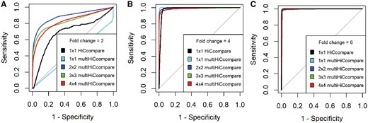
ROC analysis of the performance of multiHiCcompare and HiCCompare over various fold changes for introduced differences. The ROC curves demonstrate the increase in power in detecting differential chromosome interactions as the number of replicates per experimental condition increases from 1 to 4 compared with the performance of HiCcompare at 2, 4, 6-fold changes, panels (A), (B), (C), respectively

The performance of multiHiCcompare was also tested against the original HiCcompare, which is designed to compare two datasets. We found that both methods performed well in detecting the added differences, however, HiCcompare had a larger area under the ROC curve in cases with one replicate per experimental condition (Fig. 2). This is likely due to the limitations in calculating the dispersion factor for the negative binomial model used in multiHiCcompare when no replicates are available. Therefore, for 1×1 dataset comparison, we recommend using the original HiCcompare method, while when multiple replicates are available multiHiCcompare is more powerful at detecting true differences.

3.3 multiHiCcompare outperforms FIND

To compare the performance of multiHiCcompare with FIND, a recently published method for differential chromatin interaction detection (Djekidel et al., 2018), we generated simulated Hi-C matrices with true differences at 2, 4 and 6-fold changes (see Section 2). To test the effect of the number of replicates for each of these fold changes, we performed 2×2, 3×3 and 4×4 analyses. We found that over the range of fold changes, multiHiCcompare detected more true positives with less false positives than FIND (Supplementary Table S2) and showed a larger area under the ROC curve performance (Supplementary Fig. S3). The Matthew’s Correlation Coefficient (MCC) for multiHiCcompare was also higher than that of FIND for the majority of tested examples (Fig. 3). At the higher fold changes tested, multiHiCcompare was able to detect nearly two times the amount of true differences compared to FIND (Supplementary Table S2). These results demonstrate that multiHiCcompare outperforms FIND in the detection of differential chromatin interactions at different fold changes and different numbers of replicates.

Fig. 3.

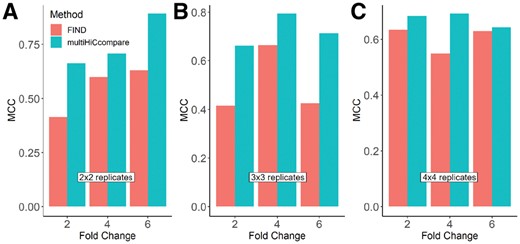
Comparison of MCC between multiHiCcompare and FIND over various fold changes and 2 × 2, 3 × 3, and 4 × 4 numbers of replicates per condition, panels (A), (B), (C), respectively. $\mathit{MCC}=\frac{\mathit{TP}\times \mathit{TN}-\mathit{FP}\times \mathit{FN}}{\sqrt{(\mathit{TP}+\mathit{FP})(\mathit{TP}+\mathit{FN})(\mathit{TN}+\mathit{FP})(\mathit{TN}+\mathit{FN})}}$

Table 2.

TFs significantly (P-value <0.05) enriched in the differentially interacting regions in HCT-116 auxin-treated cells

Transcription factor	Number of experiments	Mean logFC	Stouffer–Liptak P-value
TCF4	8	−1.07	1.38E-07
CBX3	7	−0.60	2.95E-04
EP300	1	−0.89	9.99E-04
FOSL1	1	−0.89	9.99E-04
CEBPB	1	−0.87	9.99E-04
JUND	1	−0.87	9.99E-04
RAD21	1	−0.87	9.99E-04
KMT2B	1	−0.84	9.99E-04
SRF	1	−0.83	9.99E-04
TCF7L2	1	−0.83	9.99E-04
MAX	1	−0.82	9.99E-04
TEAD4	1	−0.82	9.99E-04
USF1	1	−0.79	2.00E-03
ATF3	1	−0.79	3.00E-03
ZBTB33	1	−0.58	4.00E-03
ZC3H8	1	−0.73	6.99E-03
YY1	1	−0.78	1.10E-02
ELF1	1	−0.76	1.10E-02
EGR1	1	−0.75	2.10E-02
SMC1A	1	−0.85	4.40E-02
SP1	5	−1.13	4.41E-02
AFF4	7	−0.19	4.87E-02
MECP2	2	−0.85	4.92E-02

Note: The Stouffer-Liptak method of combining P-values (Stouffer, 1949) was used to obtain a summary P-value for each TF, as many TFs were represented by multiple datasets. ‘Number of experiments’—the number of ChIP-seq tracks supporting the enrichment, ‘Mean logFC’—the between-conditions average log fold change of regions overlapping with a TF, ‘Stouffer-Liptak p-value’—enrichment P-value summarized using Stouffer–Liptak method (sorted by).

3.4 multiHiCcompare identifies similar chromatin interaction differences detected by diffHic

We compared the performance of multiHiCcompare with the diffHic method (Lun and Smyth, 2015). We used the Hi-C data from human prostate epithelial cells (RWPE1 cells) over-expressing the ERG protein or

a GFP control, analyzed in the diffHic paper (Rickman et al., 2012). multiHiCcompare found 1752 differences (FDR < 0.05) between the ERG and GFP conditions, more than was found in the original HiCcompare analysis (Stansfield et al., 2018), yet <5737 differences (FDR < 0.05) detected by diffHic. As shown in Figure 2, multiHiCcompare might have gained some additional power over HiCcompare by making use of the two Hi-C libraries (the multiHiCcompare analysis was a 2×2 analysis, compared to the 1×1 analysis of HiCcompare). However, both HiCcompare and multiHiCcompare seem to be more conservative than diffHic. The overlap between the multiHiCcompare-detected and diffHic-detected differences was significant (1254 overlapping regions, Fisher’s exact test P-value < $2.2x{10}^{-16}$⁠). This overlap is expected as both methods utilize the same GLM framework, while multiHiCcompare applies it with respect to the distance between interacting regions. Additionally, multiHiCcompare was able to detect all but one differential interactions validated by fluorescence in situ hybridization (FISH) (Table 1), further confirming the power of multiHiCcompare in detecting biologically relevant chromatin interaction differences.

3.5 multiHiCcompare is robust to the resolution of Hi-C data

Typically, Hi-C data at higher resolution (smaller size of chromatin regions tested for interactions) have a lower dynamic range and a higher proportion of zero IFs (sparsity). To examine the effect of resolution on the performance of multiHiCcompare, we calculated the MCC at resolutions of 50, 10 and 5 KB (Supplementary Fig. S5, see Section 2). multiHiCcompare encountered some difficulties at detecting the added in differences at 2-fold changes in the very high-resolution data. However, at fold changes of 4 or greater, multiHiCcompare performed well at all resolutions. Evaluation of other performance metrics confirmed this conclusion (Supplementary Table S4). These results indicate that sparsity of the Hi-C data might hinder the detection of small differences at high resolution, but overall multiHiCcompare appears to perform well even in sparse conditions.

3.6 multiHiCcompare detects regions associated with loss of chromatin loops in auxin-treated cells

We compared data from HCT-116 cells treated with auxin to those not treated (Rao et al., 2017). The auxin treatment is thought to eliminate chromatin loops, thus changing many chromatin interactions. The untreated group contained seven samples from biological replicates 1 and 2. The auxin-treated group contained seven samples from biological replicates 1 and 2 treated with auxin for 6 h (Supplementary Table S1). All samples were jointly normalized, and differentially interacting chromatin regions were detected. The biological replicate number was entered as a covariate, and the main effect of auxin treatment was evaluated. This analysis was aimed at identifying regions associated with loss of chromatin loops.

We found a total of 417 145 differentially interacting pairs between the normal cells and the auxin treatment (FDR < 0.05). The auxin treatment is known to destroy the RAD21 protein of the cohesin complex and thus degrade chromatin looping. Therefore, we hypothesized that the regions detected by multiHiCcompare as differentially interacting should be enriched with RAD21 binding sites, and their IF should be decreased in auxin-treated condition. To test the significant differentially interacting regions for the enrichment of TF binding sites, we performed permutation tests where a random set of genomic regions of the same size as the significant regions were sampled and compared for enrichment against the significant regions. Analysis of the most significant differentially interacting regions (FDR < ${10}^{-15}$⁠) showed that they were significantly enriched for RAD21 binding sites (permutation P-value <0.001, Supplementary Table S3). Additionally, the regions enriched for RAD21 mostly exhibited lower IF values compared to the normal cells.

Notably, we detected SMC1A, another structural maintenance protein of the cohesin complex reported to be affected by the auxin treatment

(Rao et al., 2017), to be enriched in these regions (permutation P-value =0.04). Consistent with the original findings, SMC1A enriched regions also exhibited lower IF values compared to the normal cells (Supplementary Table S3). Further, consistent with the original findings, we found that HCT-116 cell-specific CTCF sites were not enriched in the detected regions. These results indicate that multiHiCcompare is capable of detecting biologically relevant differences in chromatin conformation between experimental conditions.

In addition to the expected decrease in RAD21 and SMC1A binding sites, and no change in CTCF binding, we tested whether regions differentially interacting in auxin-treated condition are enriched in other HCT-116-specific TFs (Supplementary Table S3). The rationale here was to detect other TFs that may be responsible for chromatin loop formation. Notably, we detected strong enrichment in TCF4 binding sites (Table 2), a TF previously linked to SMC3, a known component of the cohesin complex (Ghiselli et al., 2003). Furthermore, we observed enrichment of the heterochromatin protein HP1$\gamma$ (also known as CBX3) and other proteins responsible for chromatin structure (Table 2). Expectedly, chromatin IF was decreased in these regions, confirming that auxin treatment leads to loss of chromatin loops formed by the cohesin complex (Rao et al., 2017). These findings confirm that multiHiCcompare allows for deeper insights into the biology of differential chromatin interactions.

We further hypothesized that the differentially expressed (DE) genes detected in Rao et al. (2017) would be enriched within the regions detected by multiHiCcompare as differentially interacting. The list of DE genes was obtained from GEO (GSE106886) and matched with the corresponding regions by genomic coordinates. The DE genes (FDR < 0.05) were checked for enrichment within the most significant differentially interacting regions (FDR < ${10}^{-15}$⁠). We found that these genes were significantly enriched within the regions detected by multiHiCcompare (permutation P-value = $3.9\mathrm{*}{10}^{-4}$⁠). In summary, these results demonstrate that multiHiCcompare is a powerful tool to detect biologically relevant chromatin interaction differences.

3.7 multiHiCcompare detects regions associated with siRNA knockdown of CTCF

Similar to the analysis performed on the auxin-treated cells, we used multiHiCcompare to analyze an experiment of CTCF siRNA knockdown in HEK293 cells (Zuin et al., 2014). CTCF is thought to play a role in shaping the 3D organization of the genome, especially in relation to topologically associated domains (Phillips and Corces, 2009; Vietri Rudan et al., 2015), and its knockout led to the reduction of intra-domain interactions with the concurrent increase in inter-domain interactions. Thus, it was expected that knockdown of CTCF should lead to changes that can be detected by multiHiCcompare. We detected a total of 640 (FDR < 0.05) differences between the control and CTCF siRNA knockdown cells. About 448 (70%) of the differentially interacting regions had positive fold changes (mean log fold-change 2.8), potentially reflecting the increased inter-domain interactions.

Knockdown of CTCF is expected to ‘free’ its binding sites from the insulator effect of CTCF and allow the associated chromatin regions to interact. Indeed, the original study found that the promoters of genes DE after CTCF knockdown were enriched in CTCF binding sites (Zuin et al., 2014). Analysis of the significant differentially interacting regions detected by multiHiCcompare showed that they were significantly enriched for CTCF binding sites (permutation P-value <0.001, Supplementary Tables S5 and S6). Members of the cohesin complex were also found to be enriched following CTCF knockdown (Zuin et al., 2014); e.g. SMC3 was also found to be enriched in the differential regions (permutation P-value <0.001, Supplementary Table S6). These findings mirror the original results (Zuin et al., 2014), further confirming that multiHiCcompare is able to detect known biological differences in Hi-C data.

We also detected strong enrichment of POLR2A binding sites in the differential regions detected by multiHiCcompare, not reported in the original study. Notably, upregulation of polymerase genes, including POLR2A, following knockdown of TFII-I, an interacting partner of CTCF, has been noted (Marques et al., 2015). Their results suggest that the increase in inter-domain interactions followed by CTCF depletion is likely accompanied by an increase in transcription driven by RNA polymerase II. In summary, these results suggest that multiHiCcompare can confirm known and detect new findings in the comparative analysis of Hi-C data.

3.8 Runtime evaluation

In our testing, both cyclic loess and fastlo normalization methods perform reasonably equally in regards to difference detection (Supplementary Fig. S4); however, fastlo offers quicker computational speeds (Supplementary Fig. S6A). We provide cyclic loess method as a conceptually straightforward and illustrative algorithm of the joint normalization of multiple datasets and recommend fastlo as the default joint normalization method.

When compared to FIND, multiHiCcompare showed a much faster runtime. We found that FIND was extremely slow on any Hi-C matrices that were relatively complete (low proportion of zeros). For example, at resolutions of 20–5 0KB FIND runtimes were more than 72 h, while multiHiCcompare can perform a comparable analysis in under 10 min (Supplementary Fig. S6A). Thus, multiHiCcompare represents a fast and scalable method for joint normalization and detection of chromatin interaction differences.

The memory footprint expectedly increased with the increased resolution of the data and the number of replicates (Supplementary Fig. S6B). However, the memory footprint depends on sparsity of the data, hence, the high-resolution data may take less memory due to the increased sparsity. In summary, a whole-genome Hi-C data analysis can be performed on a desktop computer.

4 Discussion

As Hi-C datasets begin to be generated in multiple replicates, methods for the joint analysis of them are becoming crucial. Our methods address this need by providing a software implementation for the joint normalization of multiple datasets and the detection of differential chromatin interactions. As with any sequencing technologies, Hi-C data are unpredictably affected by technological biases, hindering the detection of chromatin interaction differences. While methods for normalization of individual Hi-C datasets have been developed (Imakaev et al., 2012; Knight and Ruiz, 2012; Lieberman-Aiden et al., 2009; Yaffe and Tanay, 2011), methods for joint normalization and comparative analysis of Hi-C data remain immature. We present the first method for jointly normalizing multiple Hi-C datasets by extending our HiCcompare loess regression-based method (Stansfield et al., 2018) and adapting the GLM-based difference detection method (McCarthy et al., 2012; Robinson et al., 2010) for the comparative analysis of multiple Hi-C datasets. multiHiCcompare can detect a priori known changes in replicate data with a low rate of false positives, and its power only increases with the increasing number of Hi-C replicates. We demonstrate that multiHiCcompare can detect biologically relevant regions associated with loss of chromatin loops in auxin-treated cells (Rao et al., 2017) and CTCF knockdown cells (Zuin et al., 2014). We believe that if replicates of Hi-C data are available, they should be used in multiHiCcompare to gain the most power in detecting chromatin interaction differences.

The diffHic method (Lun and Smyth, 2015) pioneered the use of the negative binomial distribution and the GLM framework, originally implemented in the edgeR package (Robinson et al., 2010), for the comparative analysis of two Hi-C datasets. Other tools, such as HiBrowse (Paulsen et al., 2014), diffloop (Lareau and Aryee, 2018), also utilized this framework. We further confirm the suitability of the negative binomial distribution for Hi-C data modeling (Supplementary Fig. S2) and extend the edgeR functionality with the distance-centric view of Hi-C data. Our previous results (Stansfield et al., 2018) and the current implementation demonstrate that the distance-centric analysis of Hi-C data is a powerful approach to detect true chromatin interaction differences.

Interestingly, when comparing multiHiCcompare against FIND, multiHiCcompare performed much better than FIND even when using FIND’s simulation function. This may be because FIND excels at detecting large fold changes (e.g. 10-fold or 20-fold changes) (Djekidel et al., 2018), while multiHiCcompare performs well at fold changes as small as 2. Thus, besides being much faster than FIND (see ‘Runtime evaluation’ results), multiHiCcompare is better suited for the detection of chromatin interaction differences across the whole range of fold changes.

In comparison with diffHic, multiHiCcompare showed similar performance in our analysis of the RWPE1 data. Although multiHiCcompare detected a smaller number of differences than diffHic, there was a significant overlap in the detected lists of regions. This is expected as both multiHiCcompare and diffHic use the GLM framework for difference detection but differ in the normalization approach and distance-based considerations implemented in multiHiCcompare. We feel that the distance-centric approach for joint normalization and difference detection, as implemented in multiHiCcompare, is better suited for the analysis of multiple Hi-C datasets.

In summary, the multiHiCcompare R package provides user-friendly methods for the joint normalization and comparative analysis of multiple Hi-C datasets. Our methods have been shown to perform similarly or better than other available methods. To date, multiHiCcompare is the only method for the joint normalization of multiple Hi-C datasets, which has been shown to outperform the commonly used methods for normalizing individual datasets (Stansfield et al., 2018). Finally, since multiHiCcompare is designed as a Bioconductor R package, it can be easily installed and used on all operating systems.

Funding

This work was supported by the American Cancer Society [IRG-14-192-40]; and by the National Institute of Environmental Health Sciences of the National Institutes of Health [T32ES007334].

Conflict of Interest: none declared.