Protein fold recognition based on multi-view modeling

Abstract

Motivation

Protein fold recognition has attracted increasing attention because it is critical for studies of the 3D structures of proteins and drug design. Researchers have been extensively studying this important task, and several features with high discriminative power have been proposed. However, the development of methods that efficiently combine these features to improve the predictive performance remains a challenging problem.

Results

In this study, we proposed two algorithms: MV-fold and MT-fold. MV-fold is a new computational predictor based on the multi-view learning model for fold recognition. Different features of proteins were treated as different views of proteins, including the evolutionary information, secondary structure information and physicochemical properties. These different views constituted the latent space. The $\mathrm{\epsilon }$-dragging technique was employed to enlarge the margins between different protein folds, improving the predictive performance of MV-fold. Then, MV-fold was combined with two template-based methods: HHblits and HMMER. The ensemble method is called MT-fold incorporating the advantages of both discriminative methods and template-based methods. Experimental results on five widely used benchmark datasets (DD, RDD, EDD, TG and LE) showed that the proposed methods outperformed some state-of-the-art methods in this field, indicating that MV-fold and MT-fold are useful computational tools for protein fold recognition and protein homology detection and would be efficient tools for protein sequence analysis. Finally, we constructed an update and rigorous benchmark dataset based on SCOPe (version 2.07) to fairly evaluate the performance of the proposed method, and our method achieved stable performance on this new dataset. This new benchmark dataset will become a widely used benchmark dataset to fairly evaluate the performance of different methods for fold recognition.

Supplementary information

Supplementary data are available at Bioinformatics online.

1 Introduction

The identification of the tertiary structures of proteins is of great significance in understanding the functions of proteins, protein–protein interactions, etc. Proteins in the same fold usually have similar structures and functions (Chothia and Finkelstein, 1990). Therefore, accurate prediction of protein folds is critically important for studying the structures and functions of proteins (Yan et al., 2017).

Protein fold classification is a typical taxonomy-based problem aiming to classify a query protein into one of known fold types according to its primary structure information. As a multiclass classification task, several machine learning techniques have been employed in this field (Wei and Zou, 2016). Most of these methods contain two stages: (1) feature extraction and (2) discriminative classifier construction.

For the first stage, several discriminative features have been proposed. Some researchers focused on extracting the composition of the amino acids along the protein sequences (Cheung et al., 2016). Dubchak et al. (1995) proposed a global description method for extracting the sequence features. Later, the neighbouring residues in the proteins were incorporated into the predictors. Fletez-Brant et al. (2013) proposed a Kmer-SVM method that extracted the features by calculating the frequencies of the continuous neighbouring residues in the proteins. The above features effectively capture the local discriminative information. Shen and Chou (Shen and Chou, 2006) combined the sequence-order information, hydrophobicity and hydrophilicity information using the pseudo-amino acid (PseAAC) approach to incorporate the different kinds of features. Recent studies have focused on the evolutionary information and secondary structure information, such as the Position Specific Scoring Matrices (PSSM) (Altschul et al., 1997). Dong et al. (2009) combined the auto-covariance transform and PSSM to extract the evolutionary information. Compared with the PSSM, the profile Hidden Markov Model (profile-HMM) (Remmert et al., 2012) took each position in the sequence into account to observe an insertion or deletion operation.

For the second stage, many classifiers have been applied in this field. Support Vector Machines (SVMs) have been widely used (Liu et al., 2017, 2019). Furthermore, other well-known machine learning classifiers have also been applied in this field, such as Random Forest (Dehzangi et al., 2010; Liu et al., 2016), Naive Bayes (John and Langley, 1995), ensemble learning (Chen et al., 2012a, b; Lin et al., 2013; Shen and Chou, 2006), etc. For example, Wei et al. (2015a, b) proposed a predictor called PFPA containing an ensemble learning classifier and a novel feature that combines the information from PSI-BLAST (Altschul et al., 1997) and PSIPRED (Jones, 1999). Cheung et al. (2016) proposed a method called NiRecor based on the artificial neural networks and an adaptive heterogeneous particle swarm optimizer.

In addition to the methods based on machine learning techniques, template-based methods are commonly used in protein fold recognition (Vallat et al., 2015). Template-based methods utilize the sequence homology or the structural information to match the protein sequences with a three-dimensional structure. Xia et al. (2016) utilized the sequence profile templates generated by HMM, and explored the relationship between the query sequence and template-based profiles.

Multi-view approaches utilize the information on various aspects of protein sequences from different sources (Hu et al., 2016) and integrate multiple data sources to improve the predictive performance (Ammad-ud-din et al., 2017). Each data source provides a specific view of the same protein sequence. The representation of each source is defined as a descriptor of the view that potentially encodes features of various properties. For example, the PSSM profile, PSIPRED profile, physicochemical profile and HMM profile are different data sources, and each source represents various features (Liu, 2018). In this work, we utilize the multi-view learning method to predict the protein folds. The multi-view learning method obtains the latent subspace shared with the multiple views using a subspace learning algorithm (Gu et al., 2016). Xia et al. (2010) learned the weight of each view during the learning process stage to eliminate the effects of weak views. The combination of different features has been recently shown to improve fold recognition performance. When the different features have strong dependencies, the use of combinations of features would lead to better performance because the correlated features from different descriptors are considered (Cai et al., 2014). However, the manner in which features are combined may cause the curse of dimensionality problem, and the dependency information of different features is not well explored (Gu et al., 2016; Liu et al., 2015a, b, 2018c).

Inspired by the multi-view low-rank regression model (Wen et al., 2018a, b, c, d) and the regularized least square regression (LSR) framework (Rifkin et al., 2003), we proposed a computational method for fold recognition based on the multi-view learning model called MV-fold. The method utilizes multiple input sources to learn a model. The proposed formulation assumes that only a part of the features from the input data source in each view are beneficial for protein fold recognition. The proposed method applies the ${\ell }_{2,1}$ norm regularization to extract the discriminative features (Fei et al., 2018; Nie et al., 2010; Wen et al., 2018a, b, c, d) from each view of a data source to constitute the latent subspace. Compared with the combining feature approach, the MV-fold extracts the discriminative features from the representation of each view and constitutes the latent subspace for protein fold recognition. Compared with the traditional linear regression model, the MV-fold applies the $\mathrm{\epsilon }$-dragging technique (Fang et al., 2018; Xiang et al., 2012) to enlarge the boundary distances of different protein folds. As a result, the MV-fold utilizes the latent effective features from multiple view data sources generated from the protein sequences and has greater discriminative capacity for protein fold recognition. Furthermore, an ensemble-based approach called MT-fold is proposed that combines MV-fold and two template-based methods: HHblits (Remmert et al., 2012) and HMMER (Finn et al., 2011).

2 Materials and methods

2.1 Benchmark datasets

Five benchmark datasets were used to evaluate the performance of various methods. The DD dataset (Ding and Dubchak, 2001) was obtained from the Structural Classification of Protein (SCOP) version 1.63, and contains 695 sequences with 27 folds. The four major classes in the DD dataset are α, β, α + β and α/β. The sequence identity between any two sequences is less than 35%.

The RDD dataset (Yang and Chen, 2011) is a revised version of DD dataset. Some sequences in the RDD have been updated according to the SCOP 1.75 dataset.

The extended DD called EDD (Yang and Chen, 2011) dataset from SCOP (version 1.75) contains more protein sequences than the DD dataset. EDD includes 3418 protein sequences with 27 folds.

The TG dataset from SCOP (version 1.73) contains 1612 protein sequences with 30 different folds. The dataset was proposed by Taguchi and Gromiha (Taguchi and Gromiha, 2007). The pairwise sequence identity is less than 25%.

The LE dataset derived from SCOP (version 1.37) dataset was proposed by Lindahl and Elofsson (2000). The sequence identity between any pair of sequences is less than 40%. Depending on the all-against-all comparison results of the total sequences, the dataset includes 321 sequences at the fold level (covering 38 folds). We evaluated the performance of different methods at the fold level.

Although these five benchmark datasets have been widely used to evaluate the performance of various predictors for fold recognition, they have the following disadvantages: (i) for the four benchmark datasets DD, RDD, EDD and TG, some proteins in the training set and test set are in the same superfamily. Therefore, for these proteins the fold recognition task cannot be rigorously simulated. In fact, these four benchmark datasets actually evaluate the prediction performance for an easier task: protein homology detection (Chen et al., 2018; Liu et al., 2014, 2017, 2019). (ii) Among the aforementioned five datasets, LE is the only rigorous benchmark dataset. However, it only contains 321 sequences with 38 folds. In order to overcome the two disadvantages of the existing benchmark datasets, we constructed an update, rigorous dataset (YK) based on the SCOP database (Murzin et al., 1995). YK dataset contains 4843 sequences with 82 folds. Proteins were extracted from the latest SCOPe dataset (version 2.07) genetic domain sequence subsets with less than 40% pairwise identify to each other released in 2018. The dataset was divided into three subsets, including training set, validation set and test set. To guarantee the homologous sequence redundancy between different subsets, we adopt two different strategies for homology reduction: the removal of redundant sequences at the fold level and a reduction in identical sequences (Hou et al., 2018). The first strategy splits proteins in the SCOPe 2.07 dataset into a fold-level training set, a fold-level validation set and a fold-level test set based on superfamilies, namely, the proteins from the different subsets are not in the same superfamily. Then the second strategy was to reduce the sequence redundancy between different subsets by using CD-HIT (Li and Godzik, 2006) and PSI-BLAST (Altschul et al., 1997) following the studies (Zhu et al., 2017). Following the criterion of constructing the LE dataset (Lindahl and Elofsson, 2000), we utilized CD-HIT (sequence identity: 40%) and PSI-BLAST (E-value: 1e-4) to remove the similar protein in the three subsets. After these filtering operations, the sequences identity among different subsets is less than 40%. Finally, there are 1536, 1628, 1679 sequences in training, validation and test subsets, respectively. The YK benchmark dataset is given in Supporting Information S1.

2.2 Multi-view learning model

The benchmark dataset contains n proteins ${\left\{\left(x^i,y^i\right)\right\}}_{i=1}^n$ from c types of folds based on the SCOP, where $x^i\in {\mathbb{R}}^m$ is the feature of the ith protein and $y^i$ represents its protein fold type. For a clear description of the categories of different protein folds, $y^i$ is the strict binary vector whose dimension is c. If the ith protein sequence belongs to the $j\left(j\in \left[1,\dots ,c\right]\right)$th fold, then the jth element in $y^i$ is 1 and the other elements are 0, such as ${\mathrm{y}}^i=\left[0,\dots ,\mathrm{ }0,\mathrm{ }1,\mathrm{ }0,\dots ,\mathrm{ }0\right]\in {\mathbb{R}}^c$⁠.

Suppose that n sequences on the benchmark dataset and r query sequences are represented in D views. Let ${\mathbf{X}}_{\mathrm{tr}}^{\left(d\right)}={\left[x_{\mathrm{tr}}^{1,\left(d\right)},\dots ,x_{\mathrm{tr}}^{n,\left(d\right)}\right]}^{\mathbf{T}}\in {\mathbb{R}}^{n\times m_d}\left(d\in \left[1,\dots ,D\right]\right)$ be the protein sequences in the benchmark from the dth view, where $x_{\mathrm{tr}}^{i,\left(d\right)}\in {\mathbb{R}}^{m_d}$ is the representation vector of the ith protein sequence, and $\mathbf{Y}={\left[y^1,\dots ,y^n\right]}^{\mathrm{T}}\in {\mathbb{R}}^{n\times c}$ is the strict binary matrix of the fold types of ${\mathbf{X}}_{\mathrm{tr}}^{\left(d\right)}$ sequences. The r query protein sequences are represented as ${\mathbf{X}}_{\mathrm{tt}}^{\left(d\right)}={\left[x_{\mathrm{tt}}^{1,\left(d\right)},\dots ,x_{\mathrm{tt}}^{r,\left(d\right)}\right]}^{\mathrm{T}}\in {\mathbb{R}}^{r\times m_d}\left(d\in \left[1,\dots ,D\right]\right)$ from the dth view.

Inspired by the regularized least square regression (LSR) (Rifkin et al., 2003) and robust feature selection (RFS) framework (Nie et al., 2010), we embedded the protein sequences from the D views and its corresponding label matrices in the following model:

$$\underset{{\mathbf{P}}^{\left(d\right)}}{\min }{\Vert \sum _{d=1}^D{\mathbf{X}}_{\mathrm{tr}}^{\left(d\right)}{\mathbf{P}}^{\left(d\right)}-D\mathbf{Y}\Vert }_{\mathrm{F}}^2+\mathrm{\lambda }\sum _{d=1}^D{\Vert {\mathbf{P}}^{\left(d\right)}\Vert }_{2,1}$$

(1)

where $\mathrm{\lambda }$ is a positive regularized parameter. The notation in the regularization term is the ${\ell }_{2,1}$ norm of P (Nie et al., 2010). ${\mathbf{P}}^{\left(d\right)}\in {\mathrm{R}}^{m_d\times c}$ is the transformation matrix of the $d$th view to obtain insight into the important features.

Because the traditional binary regression target has weak separability, the $\mathrm{\epsilon }$-dragging technique enforces the regression target of different classes by enlarging the margins between different categories of protein folds to the greatest extent possible. Inspired by the previous study (Xiang et al., 2012), we relaxed the strict binary into a slack variable matrix by adding a non-negative matrix $\mathbf{M}$⁠.

Now we provide an example to show how to relax the strict binary label matrix into a slack variable matrix. Let $x_1,x_2,x_3$ be the feature vectors of three training samples with three different folds. The corresponding label matrix is defined as $\mathbf{Y}=\left[\begin{array}{ccc}0& 1& 0\\ 0& 0& 1\\ 1& 0& 0\end{array}\right]\in {\mathbb{R}}^{3\hspace{0.5em}\times \hspace{0.5em}3}$ (where the first, second and third rows of $\mathbf{Y}$ denote the second, third and first folds, respectively). The distance between any two samples from different classes is $\sqrt{2}$ (i.e. the distance between the second and third samples is $\sqrt{{\left(0\hspace{0.5em}-\hspace{0.5em}1\right)}^2+{\left(0\hspace{0.5em}-\hspace{0.5em}0\right)}^2+{\left(1\hspace{0.5em}-\hspace{0.5em}0\right)}^2}=\sqrt{2}$⁠). However, the distance between two samples from different classes varies, because the protein sequences from different categories exhibit specific properties. We expect that the strict binary target matrix is relaxed into a slack matrix by applying the $\mathrm{\epsilon }$-dragging technique (Fang et al., 2018; Xiang et al., 2012). The technique drags the initial binary matrix along the different directions. More specifically, we combined the non-negative relaxation matrix $\mathbf{M}$ with the original binary matrix $\mathbf{Y}$ to form a slack matrix ${\mathbf{Y}}^{\mathrm{\text{'}}}=\left[\begin{array}{ccc}-{\mathrm{m}}_{11}& 1+{\mathrm{m}}_{12}& -{\mathrm{m}}_{13}\\ -{\mathrm{m}}_{21}& -{\mathrm{m}}_{22}& 1+{\mathrm{m}}_{23}\\ 1+{\mathrm{m}}_{31}& -{\mathrm{m}}_{32}& -{\mathrm{m}}_{33}\end{array}\right],\mathrm{ }\mathrm{s}.\mathrm{t}.{\mathrm{m}}_{\mathrm{ij}}\ge 0$⁠. The distance between any two samples from different classes is greater than or equal to $\sqrt{2}$ (i.e. the distance between the first and second samples is $\sqrt{{\left({\mathrm{m}}_{11}-{\mathrm{m}}_{21}\right)}^2+{\left(1+{\mathrm{m}}_{12}+{\mathrm{m}}_{22}\right)}^2+{\left({\mathrm{m}}_{13}+1+{\mathrm{m}}_{23}\right)}^2}\ge \sqrt{2}$⁠). As a result, the strict binary matrix $\mathbf{Y}$ is relaxed into the slack matrix ${\mathbf{Y}}^{\mathrm{\text{'}}}$ and the margins from different classes are enlarged through the non-negative matrix $\mathbf{M}$⁠.

By applying the $\mathrm{\epsilon }$-dragging technique, the strict binary matrix $D\mathbf{Y}$ in Eq. 1 is relaxed into the slack constraint so that it has more freedom to fit the regression target (Chen et al., 2012a, b; Wen et al., 2018a, b, c, d). The slack variable ${\mathbf{Y}}^{\mathrm{\text{'}}}$ is defined as:

$${\mathbf{Y}}^{\mathrm{\text{'}}}=D\mathbf{Y}+\mathbf{B}\odot \mathbf{M}$$

(2)

where the symbol $\odot$ represents a Hadamard product operator of matrices, $\mathbf{M}$ is the non-negative label matrix and $\mathbf{B}\in {\mathbb{R}}^{n\times c}$ is a constant matrix, which is defined as follows(Xiang et al., 2012):

$$B^{\mathit{ij}}=\left\{\begin{array}{c}+1,\mathrm{ }\mathrm{if}\mathrm{ }{y}^{\mathit{ij}}=1\\ -1,\mathrm{ }\mathrm{if}\mathrm{ }{y}^{\mathit{ij}}=0\end{array}\right.$$

(3)

The distances between different protein folds are enlarged in ${\mathbf{Y}}^{\mathrm{\text{'}}}$⁠. The dragging direction is related to the elements in $\mathbf{B}$⁠, where $\mathrm{“}$$+1\mathrm{”}$ is used to enlarge in the positive axis and vice versa. The elements in $\mathbf{M}$ measure the dragging distances between the margins of different protein folds’ and have more freedom to fit the regression target.

Then we propose the following objective function for multi-view fold:

$$\underset{{\mathbf{P}}^{\left(d\right)},\mathbf{M}}{\min }{\Vert \sum _{d=1}^D{\mathbf{X}}_{\mathrm{tr}}^{\left(d\right)}{\mathbf{P}}^{\left(d\right)}-D\mathbf{Y}-\mathbf{B}\odot \mathbf{M}\Vert }_{\mathrm{F}}^2+\mathrm{\lambda }\sum _{d=1}^D{\Vert {\mathbf{P}}^{\left(d\right)}\Vert }_{2,1},\mathrm{ }\mathrm{s}.\mathrm{t}.\mathbf{M}\ge 0$$

(4)

where ${\mathbf{P}}^{\left(d\right)}$ has more discriminative ability based on the ${\ell }_{2,1}$ norm. According to the previous study (Nie et al., 2010), the ${\ell }_{2,1}$ norm regularization matrix is beneficial to select the most discriminative features across all data points with joint sparsity. Therefore, the transformation matrix ${\mathbf{P}}^{\left(d\right)}$ is robust to feature selection.

Once we obtain the transformation matrix ${\mathbf{P}}^{\left(d\right)}$⁠, the predicted fold $y^v$ of the query protein sequence $x_{\mathrm{tt}}^v$ with $D$ views is calculated by the following rules:

$$j=\underset{1\le j\le \mathrm{c}}{\mathrm{argmax}}\left(y^v\right)$$

(5)

where vector $y^v=\sum _{d=1}^D{x}_{\mathrm{tt}}^{v,\left(d\right)}{\mathbf{P}}^{\left(d\right)}\in {\mathrm{R}}^c$⁠, $x_{\mathrm{tt}}^{v,\left(d\right)}$ is the feature vector of the $v$th query sequences feature of view $d\left(d\in \left[1,\dots ,D\right]\right)$⁠. Thus, the predicted protein fold utilizes the information from each view. The model obtains $c$ scores corresponding to different classes and each score is calculated by accumulating the results from $D$ views. The prediction results are directly associated with $c$ scores (summation of different views). Larger score indicates that the query sample is more likely to belong to the corresponding fold type. The solution of the proposed method is presented in Supporting Information S2.

In summary, our MV-fold model obtains different transformation matrices ${\mathbf{P}}^{\left(d\right)}$ based on the different views, and a nonnegative label matrix $\mathbf{M}$⁠. The transformation matrix ${\mathbf{P}}^{\left(d\right)}$ is powerful for selecting the discriminative features. Finally, the query sample is predicted by Eq. 5. Compared with the feature combination approaches and ensemble learning methods, MV-fold selects the discriminative features from original representations of each view and the slack variable matrix provides more freedom to fit the discriminative regression target. Therefore, MV-fold is a more robust method for protein fold recognition.

2.3 Multi-view feature representation

Protein fold recognition is a typical classification problem. MV-fold utilizes multiple views of protein sequences to predict the fold type. In this section, we will introduce several representations related to various data sources, which are treated as different views of proteins.

2.3.1 Representation of the PSI-BLAST profile

The autocross-covariance (ACC) transformation proposed by Dong (Dong et al., 2009) is used to convert the PSSM matrix to a fixed-length feature vector, whose dimension is $400\times \mathit{LG}$ (where $\mathit{LG}$ is the distance between the amino acids in the PSSM). The PSSM is generated using PSI-BLAST (Altschul et al., 1997) to search the query sequences against the NCBI’s non-redundant dataset (nrdb90). The parameters are set as ‘-j 3 –h 0.001’. In this study, the ACC is treated as the view of the representation of the PSI-BLAST profile.

2.3.2 Representation of the HHblits profile

ACC is also used to convert the HHblits profile to a fixed-length feature vector, which is denoted as ACC_HMM. HHblits based on the HMM-HMM alignment algorithm is a state-of-the-art algorithm (Remmert et al., 2012). The query sequence is searched against the database UniProt 20_2013_06 by HHblits with the parameter ‘-n 4’. The dimension of the HMM profile is $L\times 30$⁠, where the first 20 columns are the match state of amino acid emission frequencies along the sequence and the next 10 columns are seven transition frequencies and three local diversities (Xia et al., 2016). In this study, we extracted our features from the first 20 columns of amino acid emission profile information, which are similar to the 20 columns of the PSSM (Lyons et al., 2015). According to the HHblits manual (Remmert et al., 2012), the element ${\mathrm{s}}_{\mathit{ij}}$ in the profile $\mathrm{HMM}$ is calculated via $-$ $1000\times {\log }_2{s}_{\mathit{ij}}^{\mathrm{\prime }}$⁠, where ${\mathrm{s}}_{\mathit{ij}}^{\mathrm{\prime }}$ is the amino acid frequencies, and then it is transformed into ${\mathrm{s}}_{\mathit{ij}}^{\mathrm{\prime }}$ via the formula:

$${\mathrm{s}}_{\mathit{ij}}^{\mathrm{\prime }}=2^{-0.001\times {\mathrm{s}}_{\mathit{ij}}}$$

(6)

In this study, ACC_HMM is treated as the view of the representation of HHblits profile.

2.3.3 Representation of the PSIPRED profile

The statistical representation of secondary structure (⁠$\mathrm{SS}$⁠) is constructed using the PSIPRED (Jones, 1999) profile based on three states: $\mathrm{\alpha }$-helix (H), $\mathrm{\beta }$-strand (E) and random coil (C). The corresponding feature vector is represented as follows:

$$\mathrm{SS}=\left[{\mathrm{P}}_{\mathrm{C}},{\mathrm{P}}_{\mathrm{E}},{\mathrm{P}}_{\mathrm{H}},\mathrm{ }\mathrm{entropy},\mathrm{ }\mathrm{means},\mathrm{ }\mathrm{ACC},\mathrm{ }\mathrm{Bigram},\mathrm{ }\mathrm{Trigram}\right]$$

(7)

where the probabilities of the three states in the profile are calculated as follows (Xia et al., 2016):

$${\mathrm{P}}_{\mathrm{C}}=\frac{N_c}{L},{\mathrm{P}}_{\mathrm{E}}=\frac{N_E}{L},{\mathrm{P}}_{\mathrm{H}}=\frac{N_H}{L}$$

(8)

where $N_C,N_E\mathrm{ }\mathrm{and}\mathrm{ }{N}_H$ represent the occurrences of H, E and C, respectively. The entropy of the three states (Yang and Chen, 2011) is calculated as follows:

$$\mathrm{entropy}=-\left({\mathrm{P}}_{\mathrm{c}}\mathrm{l}\mathrm{n}{\mathrm{P}}_{\mathrm{C}}+{\mathrm{P}}_{\mathrm{E}}\mathrm{l}\mathrm{n}{\mathrm{P}}_{\mathrm{E}}+{\mathrm{P}}_{\mathrm{H}}\mathrm{l}\mathrm{n}{\mathrm{P}}_{\mathrm{H}}\right)$$

(9)

The means of three states H, E and C (Xia et al., 2016), the ACC (Dong et al., 2009), the Bigram (Sharma et al., 2013), the Trigram (Paliwal et al., 2014) are also incorporated into SS to represent the predicted secondary structure. In this study, the feature SS represents the view of the PSIPRED profiles.

2.3.4 Representation of the physicochemical profile

Physicochemical features impact the protein fold recognition using a template-based or ab initio folding method (Buchan and Jones, 2017). Shen and Chou (2006) utilized the physicochemical information to obtain the PseAAC. The PseAAC features are calculated via the equation (Chou, 2001)

$$\mathrm{PseAAC}=\left[P_1,\dots ,P_u,\dots ,P_{20+2\rho }\right]$$

(10)

where $P_u$ is calculated by using the equation (Chou, 2001)

$$P_u=\left\{\begin{array}{c}\frac{f_u}{{\sum }_{i=1}^{20}{f}_i+\omega {\sum }_{j=1}^{2\rho }{\tau }_j},u\in \left[1,\mathrm{ }20\right]\\ \frac{\omega {\tau }_u}{{\sum }_{i=1}^{20}{f}_i+\omega {\sum }_{j=1}^{2\rho }{\tau }_j},u\in \left[21,\mathrm{ }20+2\rho \right]\end{array}\right.$$

(11)

where $f_i$ represents the frequencies of the 20 amino acids and ${\mathrm{\tau }}_j$ is associated with the hydrophobicity and hydrophilicity information contained in the protein sequences. In this study, the feature PseAAC represents the view of the physicochemical profile. Figure 1 illustrates the hierarchical architecture of MV-fold.

Fig. 1.

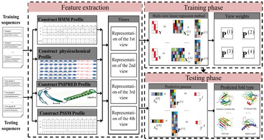
The flowchart of MV-fold. MV-fold comprises three phases: feature extraction phase, training phase and test phase. First, the proteins are embedded into feature matrices, which are constructed from different views extracted from different sources, such as the PSI-BLAST profile, the HHblits profile, the PSIPRED profile and the physicochemical profile. Second, they are fed into multi-view learning regression method to train the model. Then, the transformation matrix $\mathbf{P}$ is obtained from the model. Finally, the fold of the query protein is predicted by the transformation matrix $\mathbf{P}$⁠, and the predictive results are obtained according to the classification rule. Therefore, the MV-fold algorithm utilizes features from different views in a supervised framework

2.4 An ensemble-based method MT-fold

As shown in previous studies, fusion of various predictors is able to improve the predictive performance (Liu and Li, 2018; Liu et al., 2017, 2019, 2018a, b). Inspired by the TA-fold (Xia et al., 2016), we proposed an ensemble learning method called MT-fold that integrates dRHP-PseRA (Chen et al., 2016) and MV-fold. The dRHP-PseRA method utilizes the HHblits (Remmert et al., 2012) and HMMER (Finn et al., 2011) to search the query sequence against the training set and detect the homologous proteins. In MT-fold, when the E-values of detected homologous templates are lower than a cutoff threshold $T$ (Xia et al., 2016), the dRHP-PseRA method is used as the predictor. Otherwise, the MV-fold method is used as the predictor. Figure 2 illustrates the flowchart of MT-fold.

Fig. 2.

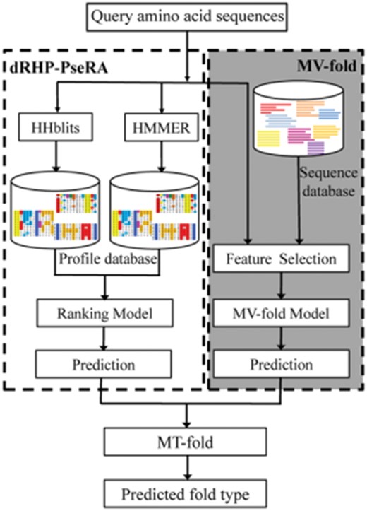
Flowchart of the MT-fold. The proposed method is divided into two parts: the dRHP-PseRA (the left module in the flowchart) and MV-fold (the right module in the flowchart with the darker background). The dRHP-PseRA searches the query sequence against the dataset using HHblits and HMMER. The MV-fold utilizes the multi-view learning model for features from different views

In the dRHP-PseRA, we utilize the HHblits (Remmert et al., 2012) and HMMER (Finn et al., 2011) to search the homology templates against the query sequence. In those methods, the profiles are generated by the Hidden Markov Model (HMM). According to the previous study (Chen et al., 2016), the two tools have various ranking hits on the same benchmark dataset, and the new framework based on those predictors improves the performance. Because HHblits (Remmert et al., 2012) and HMMER (Finn et al., 2011) share different properties, their probability hits are different. The ranking strategy is adopted to measure the different probability hits under the threshold $T$⁠. Those probability hits are sorted in descending order according to the E-values, and the proposed method chooses the probability hit with the minimum score. The performance of MT-fold is directly correlated with the cutoff threshold $T$⁠, which will be discussed in Section 3.1.

2.5 Evaluation indices

As a multiclass recognition task, the overall accuracy was employed as a metric to compare the performance of different methods. Accuracy is defined as the ratio of the number of correctly predicted proteins to the number of total proteins by using equation (Dong et al., 2009):

$$\mathrm{Accuracy}=\frac{\mathit{CN}}{N}\times 100\mathrm{\%}$$

(12)

where $\mathit{CN}$ denotes the number of the protein samples which are predicted correctly, and $N$ is the total number of query samples of the test dataset.

The standard deviation (SD) is used to measure the dispersion of the data from its mean of the Accuracy scores of $k$-fold cross-validation (Tibshirani et al., 2002):

$$\mathrm{SD}=\sqrt{\frac{1}{N}{\sum }_{i=1}^N{\left(x_i-\overline{x}\right)}^2}\times 100\mathrm{\%}$$

(13)

where $x_i$ denotes the value of predicted accuracy of each fold in the cross-validation and $\overline{x}$ is the mean of the accuracies.

3 Results and discussion

3.1 Determination of parameter and cross-validation

There are two kinds of parameters in the MV-fold method: the parameters associated with the four view data sources, and the parameter $\mathrm{\lambda }$ associated with the multi-view learning model. In this study, the parameters associated with the four views data sources were optimized on RDD dataset via the 10-fold cross-validation. These parameters were optimized on the validation set, which is dependent with the training and test sets. The optimized values of these parameters are shown in Table 1, which were also used for other benchmark datasets to reduce the risk of the over-fitting. The parameter $\mathrm{\lambda }$ associated with the multi-view learning model was optimized on the validation set fully independent with the training and test sets on different benchmark datasets, respectively. 10-fold cross-validation was used for DD, RDD, EDD and TG, and 2-fold cross-validation and 3-fold cross-validation were used for LE and YK, respectively. For more details of the parameter optimization process and the values, please refer to the Supporting Information S3.

Table 1.

The parameter values of different views

Different views	PSI-BLAST profile	HHblits profile	PSIPRED profile	physicochemical profile
Values	$\mathit{LG}=1$	$\mathit{LG}=5$	$\mathit{LG}=9$	$\mathrm{\rho }=5,\omega =0.5$

For MT-fold, there is an additional parameter $T$ for combining MV-fold and dRHP-PseRA, which was optimized on EDD dataset, and the best performance was achieved when $T$ was equal to 0.5. The impact of this parameter on the performance of MT-fold is shown in Supplementary Figure S1 in Supporting Information S3. This value was used for all benchmark datasets to avoid the risk of over-fitting.

3.2 The performance and properties of MV-fold

MV-fold utilizes four views to construct the predictor, including ACC, ACC_HMM, SS and PseAAC. MV-fold was compared with predictors based on four traditional classifiers (LIBSVM with RBF kernel, KNN, Random Forest and RFS) to show the performance of the multi-view learning model. We linearly combine the descriptors from different views with the same parameters, and then this combination of features is fed into those traditional classifiers. The prediction accuracies of those methods are listed in Table 2.

Table 2.

The performance of MV-fold and other classifiers in terms of accuracy (cf. Eq. 12)

Method	DDa	RDDa	EDDa	TGa	LEb	YKc
MV-fold	83.5%	91.7%	94.8%	86.2%	46.6%	46.4%
LibSVM	69.5%	81.3%	86.5%	70.5%	41.4%	41.9%
KNN(k=1)	61.2%	73.2%	74.4%	53.0%	33.3%	30.5%
Random Tree	72.7%	82.9%	89.8%	76.0%	38.9%	40.8%
RFS	77.0%	85.5%	90.5%	81.9%	40.4%	43.9%

a

From 10-fold cross-validation.

b

From 2-fold cross-validation.

c

From 3-fold cross-validation.

As discussed in Section 2.1, the four datasets DD, RDD, EDD and TG are mainly used to evaluate the performance of a predictor for protein homology detection, and the two datasets LE and YK are used to evaluate the performance for fold recognition. From Table 2 we can obviously see that MV-fold outperforms the other predictors on all the 6 datasets, indicating that the multi-view learning model is effective for both fold recognition and homology detection. Compared with the traditional predictors utilizing a combination of features, MV-fold selects the significant features of each view by using the transform matrix $\mathbf{P}$ and those features are critical for the predictive performance improvement. Compared with the RFS method which utilizes the linear regression model and selects the discriminative features using the ${\ell }_{2,1}$ norm, the proposed MV-fold method applies the $\mathrm{\epsilon }$-dragging technique to enforce the regression targets of different categories by moving along mutually opposite direction to enlarge the margin distances between different protein folds. This technique is more powerful than other existing linear regression methods, such as RFS. Therefore, MV-fold outperforms traditional predictors.

Because only some features in each view are used for the prediction, we selected the discriminative features to constitute the latent subspace, where the selected features are very important for the prediction. Then, the new samples are predicted by the discriminative features through the transformation matrices. According to the previous study, the ${\ell }_{2,1}$ norm has a row-sparsity property, which is associated with the discriminative features (Nie et al., 2010). In the MV-fold, we utilized the regularized ${\ell }_{2,1}$ norm to obtain the comprehensive projection matrix $\mathbf{P}$⁠. Figure 3 shows the projection matrices of the special views obtained by the proposed method. Figure 3a shows the first 125 rows of $\mathbf{P}$⁠. We calculated the value of each row in the former 125 rows of $\mathbf{P}$ by using the ${\ell }_2$ norm. Most of the elements displayed in Figure 3b have values near zero. The transformation matrix $\mathbf{P}$ obtained from the MV-fold method exhibits the row-sparsity property. The nonzero elements of the transformation matrix are directly correlated with the selected features, which have great discriminative power. The features in the transformation matrix are interpretable, and the ${\ell }_{2,1}$ norm has the ability to select the most discriminative features from original data for feature selection.

Fig. 3.

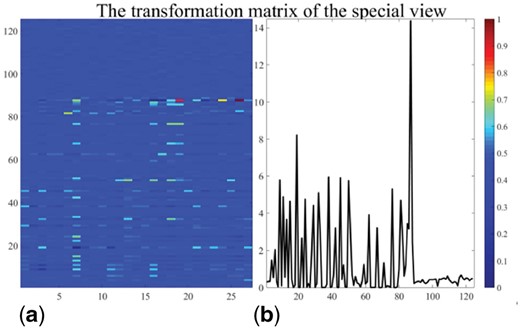
The transformation matrix of the special view on the RDD dataset. The subfigure (a) shows the transform matrix ${\mathbf{P}}^{\left(d\right)}$ corresponding to the special view. The first 125 rows of the transformation matrix are shown. We calculated the values of each row in ${\mathbf{P}}^{\left(d\right)}$ by using the ${\ell }_2$ norm to show the row-sparsity property. The values of different rows are displayed in the subfigure (b).

In MV-fold, different views of proteins provide complicated projection matrices. Different feature groups without data integration are fed into MV-fold for the four datasets, including DD, RDD, EDD and TG, to investigate the contributions of four views to the performance of MV-fold. Supplementary Figure S2 in Supporting Information S3 shows the performance of different views on the four datasets. The accuracy of MV-fold is improved by utilizing the different view feature groups. In each view, we extracted the discriminative features to constitute the latent subspace and then predicted the query protein sequence in the latent subspace.

In our experiments, the multi-view learning model selected the important features by using the ${\ell }_{2,1}$ norm term and achieved a more discriminative regression target by using the $\mathrm{\epsilon }$-dragging technique.

3.3 The performance of MT-fold

As an ensemble method, MT-fold combines MV-fold and dRHP-PseRA. In MT-fold, the E-value from dRHP-PseRA is used to evaluate the homologous sequences between the templates and query sample. The results of MT-fold on the six benchmark datasets are shown in Table 3, and MT-fold obviously outperforms the MV-fold and dRHP-PseRA methods on the six benchmark datasets.

Table 3.

The performance of proposed methods on different datasets in terms of accuracy (cf. Eq. 12) and SD (cf. Eq. 13)

Dataset	MV-fold	dRHP-PseRA	MT-fold
DDa	83.5±3.4%	82.4±2.4%	88.2±3.3%
RDDa	91.7±2.2%	85.5±4.0%	96.7±2.1%
EDDa	94.8±1.5%	93.9±1.3%	97.1±1.4%
TGa	85.1±2.4%	85.4±2.9%	92.0±3.3%
LEb	46.6±2.2%	37.3±0.3%	54.1±4.9%
YKc	46.4±4.8%	34.1±4.5%	50.5±4.4%

a

From 10-fold cross-validation.

b

From 2-fold cross-validation.

c

From 3-fold cross-validation.

3.4 Comparison with other methods for protein homology detection

The performance of MV-fold and MT-fold was compared with other state-of-the-art methods for protein homology detection, including the ACCFOLD (Dong et al., 2009), Taxfold (Yang and Chen, 2011), PFPA (Wei et al., 2015a, b), HMMFold (Lyons et al., 2015), NiRecor (Cheung et al., 2016), SVM-fold (Xia et al., 2016) and TA-fold (Xia et al., 2016) to show the effectiveness of our methods. The performance of these methods is described in Table 4 and Supplementary Figure S3 in Supporting Information S3. As shown in Table 4, MT-fold and MV-fold obviously outperform other state-of-the-art methods for protein homology detection on the four benchmark datasets.

Table 4.

The performance of MV-fold, MT-fold and other taxonomy methods for protein homology detection via 10-fold cross-validation on the four datasets, including DD RDD, EDD and TG in terms of accuracy (cf. Eq. 12)

Method	DD	RDD	EDD	TG
ACCFold_ACC	70.1%	73.8%	85.9%	66.4%
Taxfold	71.5%	83.2%	90.0%	NA
PFPA	73.6%	NA	92.6%	NA
HMMFold	75.8%	NA	93.8%	86.0%
NiRecor	81.2%	NA	91.7%	84.6%
SVM-fold	77.3%	90.0%	94.5%	86.5%
TA-fold	79.9%	93.2%	97.1%	92.7%
MV-fold	83.5%	91.7%	94.8%	85.1%
MT-fold	88.2%	96.7%	97.1%	92.0%

The multi-view model exhibits better performance than the data integration frameworks, such as Tax-fold and SVM-fold. These methods embed comprehensive features from different profiles into SVM classifiers. The transformation matrices corresponding to different views effectively improve the performance of data integration by selecting the discriminative features from a single view, and the $\mathrm{\epsilon }$- dragging technique is more reliable for fitting the regression targets. The MT-fold method combines the advantages of the MV-fold and dRHP-PseRA methods. Therefore, MT-fold is better than the MV-fold method.

3.5 Comparison with other methods for protein fold recognition

The proposed methods were further tested on the LE dataset to evaluate their performance for protein fold recognition. Their performance was compared with other 11 state-of-the-art methods, including HHpred (Söding, 2005), FFAS-3D (Xu et al., 2014), SPARKS-X (Yang et al., 2011), HH-fold (Xia et al., 2016), TA-fold (Xia et al., 2016), FOLDpro (Cheng and Baldi, 2006), DN-Fold (Jo et al., 2015), RFDN-Fold (Jo et al., 2015), RF-fold (Jo and Cheng, 2014), DeepFR (with strategy 1) (Zhu et al., 2017) and dRHP-PseRA (Chen et al., 2016).

The experimental results of different methods on LE dataset are listed in Table 5, showing that MT-fold outperforms all the other compared methods. MT-fold is able to capture the discriminative features of different folds, which would provide useful information for researchers who are interested in exploring the characteristics of protein folds.

Table 5.

The performance of MV-fold, MT-fold and other methods for protein fold recognition on LE dataset via 2-fold cross-validation in terms of accuracy (cf. Eq. 12)

Methods	LE
HHpred	25.2%
FFAS-3D	35.8%
SPARKS-X	45.2%
HH-fold	42.1%
TA-fold	53.9%
FOLDpro	26.5%
DN-Fold	33.6%
RFDN-Fold	37.7%
RF-fold	40.8%
DeepFR	44.5%
dRHP-PseRA	34.9%
MV-fold	46.6%
MT-fold	54.1%

Compared with the results listed in Tables 4 and 5, we can obviously observed that for the three common methods (TA-fold, MV-fold and MT-fold), their performance on the four benchmark datasets (DD, RDD, EDD and TG) is obviously higher than that of on the LE benchmark dataset. In order to explore the reasons, we further analyzed the five benchmark datasets, and found that for the four benchmark datasets (DD, RDD, EDD and TG), some proteins in the training set and test set are in the same superfamily. For example, on the TG benchmark dataset, 25 protein sequences from the Cytochrome C fold have the same superfamily a.3.1 according to the SCOPe 2.07. Therefore, the performance of the three predictors on the four benchmarks was overestimated. In fact, these four datasets are actually used to evaluate the performance for protein homology detection, an easier task than protein fold recognition. In contrast, the LE dataset is the only rigorous dataset for fold recognition. We constructed an update and rigorous dataset (YK) and the performance of MV-fold and MT-fold was evaluated on the YK dataset. A 3-fold cross-validation was adopted, and the whole dataset was divided into three subsets at the fold-level. In other words, the proteins in the training, validation and test datasets come from different superfamilies. The results are listed in Table 6 and show that MT-fold can achieve stable performance in comparison with the results on LE dataset.

Table 6.

The performance of MV-fold and MT-fold on YK dataset via 3-fold cross-validation in terms of accuracy (cf. Eq. 12)

Methods	YK
dRHP-PseRA	34.1%
MV-fold	46.4%
MT-fold	50.5%

4. Conclusion

Protein fold recognition and homology detection is important for understanding the protein structures (Wei et al., 2015a, b; Zou, 2016). In this paper, we introduce two novel recognition algorithms: MV-fold and MT-fold. MV-fold employs the multi-view learning model based on the discriminative linear regression framework. MT-fold combines the MV-fold and the dRHP-PseRA. The MV-fold utilizes four features as representations of the corresponding views and extracts significant features from each view of the data source. Then, the new samples are mapped into the views-agreement space, and their protein folds are predicted based on the selected discriminative features obtained by the transformation matrices. Unlike conventional linear regression methods, the MV-fold applies the $\mathrm{\epsilon }$-dragging technique by enlarging the margins between different categories of protein folds. As an ensemble method, MT-fold outperforms MV-fold. In the future, we will try to accelerate our methods with a parallel framework, such as Map-Reduce (Zou et al., 2014). It can be anticipated that the multi-view framework will have many potential applications in the field of bioinformatics, such as DNA binding protein identification (Zhang and Liu, 2017), protein remote homology detection (Chen et al., 2017; Liu et al., 2015a, b, 2018c), disordered region detection (Liu et al., 2018a, b), protein sequence analysis (Song et al., 2018; Wang et al., 2016), etc.

Acknowledgments

The authors are very much indebted to the three anonymous reviewers, whose constructive comments are very helpful for strengthening the presentation of this paper.

Funding

This work was supported by the National Natural Science Foundation of China (No. 61672184, 61822306), Fok Ying-Tung Education Foundation for Young Teachers in the Higher Education Institutions of China (161063), Scientific Research Foundation in Shenzhen (Grant No. JCYJ20150626110425228, JCYJ20170307152201596), Guangdong Province High-Level Personnel of Special Support Program under Grant 2016TX03X164 and 2016TQ03X618.

Conflict of Interest: none declared.