ClusterMap: compare multiple single cell RNA-Seq datasets across different experimental conditions

Abstract

Motivation

Single cell RNA-Seq (scRNA-Seq) facilitates the characterization of cell type heterogeneity and developmental processes. Further study of single cell profiles across different conditions enables the understanding of biological processes and underlying mechanisms at the sub-population level. However, developing proper methodology to compare multiple scRNA-Seq datasets remains challenging.

Results

We have developed ClusterMap, a systematic method and workflow to facilitate the comparison of scRNA-seq profiles across distinct biological contexts. Using hierarchical clustering of the marker genes of each sub-group, ClusterMap matches the sub-types of cells across different samples and provides ‘similarity’ as a metric to quantify the quality of the match. We introduce a purity tree cut method designed specifically for this matching problem. We use Circos plot and regrouping method to visualize the results concisely. Furthermore, we propose a new metric ‘separability’ to summarize sub-population changes among all sample pairs. In the case studies, we demonstrate that ClusterMap has the ability to provide us further insight into the different molecular mechanisms of cellular sub-populations across different conditions.

Availability and implementation

ClusterMap is implemented in R and available at https://github.com/xgaoo/ClusterMap.

Supplementary information

Supplementary data are available at Bioinformatics online.

1 Introduction

Single cell RNA sequencing (scRNA-Seq) is an advanced technology that sheds light on the high-resolution heterogeneity and dynamics of the transcriptome. Following massive studies on cell sub-types under static conditions, researchers are starting to pursue high-resolution mechanisms of different biological processes. With more complicated experimental designs that include different treatment conditions, different developmental time points, or different tissue types, researchers seek information on heterogeneous changes of sub-populations of cells.

There are many existing methods and packages for identification of cellular sub-types, developmental trajectory and differential expression analysis in single cell expression analysis (Angerer et al., 2016; Bacher and Kendziorski, 2016; Finak et al., 2015; Haghverdi et al., 2015; Hart et al., 2015; Ji and Ji, 2016; Kharchenko et al., 2014; Macosko et al., 2015; Pierson and Yau, 2015; Trapnell et al., 2014). However, most of them are either restricted to one single cell dataset or focused on batch effect correction across datasets (Haghverdi et al., 2018; Shaham et al., 2017). Methods for directly comparing multiple scRNA-Seq datasets across biological conditions to study heterogeneity of changes of cell sub-types are still under development. One of the current common strategies is to combine multiple datasets and then analyze it as a single dataset, which might miss critical information at the cell sub-type level. The other typical approach is to check the expression of one or a few known marker genes and use that to match the corresponding sub-groups (Kang et al., 2018; Pal et al., 2017; Zheng et al., 2017). This manual step biases the matching towards several pre-selected genes and might not be accurate. Some recently published methods attempt to address similar issues (Butler et al., 2018; Kiselev et al., 2018). Butler et al. (2018) attempt to align scRNA-seq datasets using canonical-correlation analysis (CCA) so that shared subpopulations across datasets can be compared directly. CCA analysis resembles batch effect removal methods, which assume the overall differences among samples are technical. However, the batch effects are always confounded with the biological conditions and hard to be removed. Besides, CCA may reduce the difference of some sub-groups within the same sample. Scmap (Kiselev et al., 2018) maps a single scRNA-seq sample to reference datasets to annotate the new dataset, which assign cells to known populations as a traditional classification problem. Scmap maps each cell to either the cluster centroid or the nearest cell in the reference. Scmap uses absolute expression value as the cluster centroid for cell assignments. Although it claimed that scmap can overcome batch effect, when the batch effect shifts the expression dramatically, scmap may assign the cells to a wrong cluster. We will show this in the following case study.

Here we present ClusterMap, a tool to match and compare multiple single cell expression datasets at the cluster level. ClusterMap uses binary expression patterns of marker genes of each sub-group as features for comparison. The binary marker genes are relatively different between sub-groups within each sample, which will overcome the batch effects directly. Besides, for the particular multi-sample matching problem, we developed a purity tree cut method to partition the sub-groups of samples into new matched groups. ClusterMap provides the quantification indexes ‘similarity’ and ‘separability’ to assess the confidence of the matching and the changes within each sub-group across samples. As a systematic workflow, ClusterMap also provides convenient visualization of the results.

Overall, ClusterMap provides an easy-to-use and reliable workflow to compare multiple single cell RNA-Seq datasets with complex experimental designs: across various treatments, across time points and across tissues. We demonstrate the usage and advantages of ClusterMap in several case studies and compare it to CCA and scmap analysis. Our analysis shows precise alignment of the sub-groups in different conditions, accurate characterization of differences between matched sub-groups, and identification of unique sub-groups of cells. Our method is a valuable tool for comparison of complex scRNA-seq datasets with multiple treatments or timepoints and offers a deeper understanding of the biological processes at the cellular sub-population level.

2 Materials and methods

2.1 Workflow overview

ClusterMap focuses on the analysis of sub-group matching and comparison across single cell RNA-Seq samples. ClusterMap analysis is based on the pre-analysis of each individual dataset. The sub-group definitions, identification of marker genes for each group, and dimension reduction are generated in the pre-analysis step and used as input to ClusterMap. This step can be achieved using the Seurat package (Macosko et al., 2015), 10× Genomics Cell Ranger, or other single cell analysis methods. The summarized workflow of ClusterMap is shown in Figure 1.

Fig. 1.

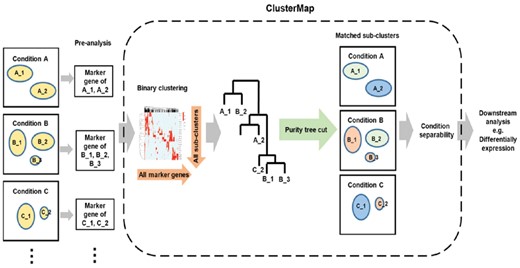
Diagram of the workflow of ClusterMap

ClusterMap uses identified marker genes for each sub-group of each sample as the basic input to match clusters. Through hierarchical clustering analysis of the binary expression patterns of marker genes and the purity tree cut method, the sub-groups identified in the pre-analysis step for each individual dataset will be matched and grouped together with the most similar sub-groups in the other samples. This could result in groups matching in a one-to-multiple, multiple-to-multiple, or singleton fashion, which enables the detection of unique or novel sub-types of cells. The similarity of the matched groups is extracted from the clustering results. With the number of cells (cell percentage) in each sub-group as an additional input, ClusterMap generates a Circos plot (Kryzwinski et al., 2009; Gu et al., 2014) to show matched sub-groups between datasets and the compositional changes of the sub-groups across datasets (Fig. 3E). The chords link the matched sub-groups. Different chord colors indicate different regroups, while the transparency of the chord color indicates the similarity of matched groups (more transparent indicates less similar). The widths of the black sectors represent the percentage of the number of cells in each sample. Thus, the sub-population size change is reflected by comparing the sector size of linked groups. New cluster labels will be assigned according to the cluster matching results. If 2D coordinates from a dimensional reduction t-distributed Stochastic Neighbor Embedding (t-SNE) plot are provided for each cell, ClusterMap will re-color the plot to coordinate the colors for the matched groups in different samples (Figs 1 and 4A–C). This will facilitate the visualization of the matching sub-groups. Finally, ClusterMap will calculate the separability to characterize the property changes across samples for each set of matched groups (Figs 1 and 3F). This measurement enables quick and unbiased identification of the most highly affected cell sub-types across all the sample comparisons.

Following ClusterMap, differential expression analysis for the most affected group might be a common following step to investigate the difference further. Since many methods have been well established, such as DESeq2, SCDE and BASiCS (Kharchenko et al., 2014; Love et al., 2014; Soneson and Robinson, 2018; Vallejos et al., 2016), this aspect of analysis is not included in ClusterMap.

2.2 Binary hierarchical clustering

The sub-groups are matched using hierarchical clustering (Figs 1 and 3D). The presence (binary) of the marker genes in each group is used to measure the distance between the sub-groups across the samples. The union of all marker genes is used for clustering. We construct a matrix showing expression of all identified marker genes for all sub clusters across multiple datasets. The value of a marker gene is assigned as 1 or 0, depending on whether this gene is identified as the marker gene for a specific sub-cluster or not. Hierarchical clustering of this binary matrix is performed using average linkage and Jaccard distance. The similarity of the matched groups is defined as 1 minus the height of the merging node of the matched groups in the dendrogram, which is the Jaccard index at that node (Figs 1 and 3F). It measures the percentage of marker genes that overlap between the matched groups.

Using the binary value of marker genes is superior to using the actual expression level to match sub-groups across samples for a few reasons. First, the expression level of a gene across cells or samples may vary a lot under different conditions. Without proper normalization methods, its direct use will be subject to noise. Binarizing expression tolerates global shifts of the transcriptome, or possible systematic batch effect across datasets. Second, given the high drop-out rate of current scRNA-seq technology, using binary values is more reliable and robust. Consequently, using Jaccard distance as a measure of similarity of sub-groups is more reasonable than Euclidian distance.

2.3 Purity tree cut

The purity tree cut algorithm is designed to match the most similar sub-groups from different samples, while avoiding forming large clusters of sub-groups that come from the same sample. Traditional clustering assessment methods, such as the Elbow method, Silhouette index, Dunn index or other indexes, are not optimal for this purpose, because the origin of samples is disregarded. Our algorithm decomposes the clustering dendrogram from the bottom-up based on both the distance between branches and the purity of the node (Fig. 2A). The purity tree cut algorithm decides to keep or trim a given node by checking the following three aspects.

Fig. 2.

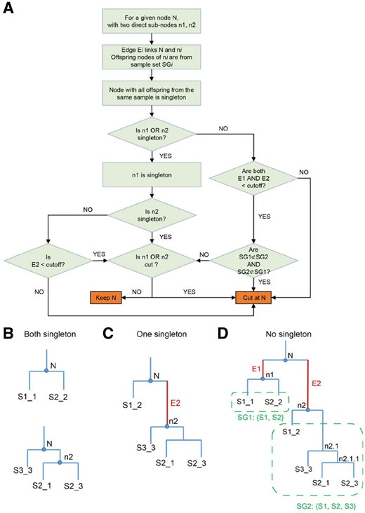
Diagram of the dendrogram tree cut algorithm. (A) Purity tree cut algorithm. Examples of the three conditions in the tree cut. (B) Two singletons. (C) One singleton. (D) No singleton

First, we consider the purity of the node. In a dendrogram, the sample set of a node is the set of samples that all its offspring nodes come from. If all the offspring nodes are from the same sample (only one sample is in its sample set), then the node is considered pure, and treated as a singleton node. For example, in Figure 2D, the offspring of node n1 are S1_1 and S2_2. They are from sample S1 and S2. Thus, the sample set of node n1 is {S1, S2} and n1 is not a pure node. For node n2.1.1, the offspring S2_1 and S2_3 are from the same sample S2, thus n2.1.1 is a pure node and is treated as a singleton node (Fig. 2D).

Second, we consider the edge length of the two branches. The edge length in a dendrogram is the height difference between the upper node (such as N) and the lower node (such as n1 in Fig. 2D). An edge length cutoff controls whether two branches of a node should be merged into one group. If an edge is longer than the cutoff, then one branch is quite different from the other branch, and it will not be merged. The default cutoff is set to 0.1, so <10% of the marker genes can be different in order to continue merging two branches.

Third, we consider the overlap between the sub-samples of the two branches.

We search through all the nodes in the dendrogram from the bottom up. For a given node N with two direct sub-nodes n1 and n2, and edges E1 and E2, N will be kept only under one of the three conditions:

1. n1 and n2 are both singleton or pure (Fig. 2B).

2. n1 is singleton or pure, AND the edge E2 is shorter than the edge cutoff, AND n2 is not cut based on the sub-nodes of n2 (Fig. 2C).

3. Both edge E1 and E2 are shorter than the edge cutoff, AND the two sample sets SG1 and SG2 are not subsets of each other (SG1⊄SG2 AND SG2⊄SG1), AND none of n1 or n2 is trimmed (Fig. 2D).

In all other conditions, node N will be removed, and n1 and n2 will form two different groups. Using Figure 2D as an example, based on condition 1, node n1 will be kept, because both S1_1 and S2_2 are singletons. So S1_1 and S2_2 are matched and form a new group Node n2.1.1 is equivalent to a singleton, thus node n2.1 will be kept with two singleton sub-nodes based on condition 1. S2_1, S2_3 and S3_3 will form one matched group. Due to condition 2, node n2 will be trimmed if the edge between n2 and n2.1 is longer than the cutoff, and S1_2 will not be grouped together with the other branch. Node N violates condition 3 and will be trimmed, because SG1 is a subset of SG2.

We generated a random tree with four samples and 10 sub-groups in each sample to test the purity tree cut algorithm (Supplementary Fig. S1A). The results were as expected, similar sub-groups are grouped together but avoid forming big groups from the same sample (Supplementary Fig. S1B). If we increase the edge cutoff, more sub-groups merge into bigger groups but with lower similarity (Supplementary Fig. S1C). A random tree of 10 samples with 10 sub-groups each was shown as well (Supplementary Fig. S2A and B). We also used our method on a real dataset with T cells from 12 patients. Each sample contains about 12 T cell sub-types (Zhang et al., 2018). We matched the pre-defined sub-types using marker genes and purity tree cut. The majority of the corresponding sub-types were matched (Supplementary Fig. S2C and Supplementary Table S1), except the sub-types with less distinct boundaries in the original definition (Supplementary Fig. S9B, Zhang et al., 2018). The following case studies also suggest that the tree cutting results match the underlying biological expectations.

The purity tree cut algorithm will match a group with its most closely related sub-group from another sample. Whether the matched group is best or not is relative to other groups. Thus, sub-groups with low similarity may be grouped together when there are no better options. It’s reasonable to filter out low similarity groups and treat them as unmatched groups for downstream analysis. Refining the marker genes list might improve the similarity between matched groups.

2.4 Separability

We propose ‘separability’ to quantify the difference in matched sub-groups using the expression level of genes after dimensional reduction. Separability can be defined for the entire transcriptome or the set of highly variable genes from the pre-analysis. Separability is defined based on the distance of the K-nearest neighbors intra- and inter-samples in a 2D space including all cells from datasets (2D space such as the combined t-SNE plot, Supplementary Fig. S1D). For each new group and each pair of two samples in the group, the separability index is defined as the median difference of intra- and inter-sample distance of each cell within the new group. Assume ${\mathbf{C}}_{\mathrm{i}}^{\left(1\right)}$ is a cell from sample 1 with n1 cells, we search for the k nearest cells to ${\mathbf{\text{C}}}_{\mathrm{i}}^{\left(1\right)}$ for all cells within sample 1, represented by ${\mathbf{\text{C}}}_{\text{ik}}^{\left(1\right)}$⁠. We also search for the k nearest cells to ${\mathbf{\text{C}}}_{\mathrm{i}}^{\left(1\right)}$ for all cells within sample 2, represented by ${\mathbf{\text{C}}}_{\text{ik}}^{\left(2\right)}$⁠, sample 2 with n2 cells. We define

Intra-sample distance for cell ${\mathbf{\text{C}}}_{\mathrm{i}}^{\left(1\right)}$ as

$${\mathbf{D}}_{\mathbf{i}}^{\mathbf{Intra}}=\mathbf{media}{\mathbf{n}}_{\mathbf{k}}\left|\left| {\mathbf{C}}_{\mathbf{i}}^{(1)}– {\mathbf{C}}_{\mathbf{i}\mathbf{k}}^{(1)}\right|\right|, \hspace{0.5em}\mathbf{for} \mathbf{k}=\mathbf{1}, \mathbf{2}, \mathbf{3}, \dots , \mathbf{K}$$

Inter-sample distance for cell ${\mathbf{\text{C}}}_{\mathrm{i}}^{\left(1\right)}$ as

$${\mathbf{D}}_{\mathbf{i}}^{\mathbf{Inter}}=\mathbf{media}{\mathbf{n}}_{\mathbf{k}}\left|\left| {\mathbf{C}}_{\mathbf{i}}^{(1)}– {\mathbf{C}}_{\mathbf{k}}^{(2)}\right|\right|, \mathbf{for} \mathbf{k}=1, \mathbf{2}, \mathbf{3}, \dots , \mathbf{K}$$

The separability of sample1 to sample2 as

$$\mathbf{SEP}1=\mathbf{media}{\mathbf{n}}_{\mathbf{i}}({\mathbf{D}}_{\mathbf{i}}^{\mathbf{Inter}}– {\mathbf{D}}_{\mathbf{i}}^{\mathbf{Intra}}, \mathbf{for} \mathbf{i}=\mathbf{1}, \mathbf{2}, \mathbf{3}, \dots , \mathbf{n}\mathbf{1}$$

For every cell in the second sample, ${\mathbf{\text{C}}}_{\mathrm{j}}^{\left(2\right)}$⁠, the separability of each cell is calculated similarly. The separability of sample2 to sample1 as

$$\mathbf{SEP}\mathbf{2}=\mathbf{media}{\mathbf{n}}_{\mathbf{j}}({\mathbf{D}}_{\mathbf{j}}^{\mathbf{Inter}}– {\mathbf{D}}_{\mathbf{j}}^{\mathbf{Intra}}), \mathbf{for} \mathbf{j}=\mathbf{1}, \mathbf{2}, \mathbf{3}, \dots , \mathbf{n}\mathbf{2}$$

Then the separability of sample1 versus sample2 in this new group is defined as

$$\mathit{Separability}=\mathbf{mean} \mathbf{\left(}\mathbf{SEP}\mathbf{1}, \mathbf{SEP}\mathbf{2}\mathbf{\right)}$$

Using median instead of mean will reduce variation due to outliers. Increasing K will improve accuracy but slow down computation. Practically, the default K is 5, and using K > 20 improves the accuracy only slightly. Separability is calculated for a pair of samples. Pairwise separability will be measured if there are more than two samples.

3 Results

3.1 Epithelial cells in different estrus cycle phases

We first applied ClusterMap to compare sub-population changes in two different biological phases using the epithelial datasets that were generated in the study of Pal et al. (2017). Cells were collected from mammary glands of adult mice during different phases of the estrus cycle. By pooling the glands from two mice, scRNA-Seq of 2729 epithelial cells in estrus and 2439 cells in diestrus was performed using the 10× Chromium platform.

We first analyzed individual datasets and identified marker genes for 13 sub-groups in diestrus and 10 sub-groups in estrus (Fig. 3A and B). To match between the set of 13 diestrus groups and the set of 10 estrus groups, ClusterMap clustered the sub-groups based on all marker genes (Fig. 3C). The clustering dendrogram (Fig. 3D) was decomposed using purity tree cut algorithm to form new matched groups (Section 2, Fig. 3F). Matched sub-groups are connected with chords in the Circos plot (Fig. 3E). The similarity of matched groups ranges from 0.29 to 0.65 (Fig. 3F) and is shown by the transparency of the chords in the Circos plot. This indicates that the sub-groups were matched with different percentages of marker genes overlapped. The population size changes were shown by the cell percentage in Figure 3F and indicated by the black sectors in the Circos plot. The Regroup 2, 3 and 9 were obviously increased in estrus (14–24, 8–35 and 1–5%, respectively, Fig. 3F). ClusterMap recolored the t-SNE plots of each sample (Fig. 4A and B) and the combined samples (Fig. 4C) with the new group assignments. Matched groups are shown in the same color and with the same new group label. Note that cells with the same color were clustered together in the combined sample, which confirmed our matching results. Additionally, the separability for each new group further highlighted the most affected sub-groups. The higher the separability value, the more drastically the group was changed, such as Regroup 6, 8 and 3, in addition to the groups unique to one sample (Fig. 3F).

Fig. 3.

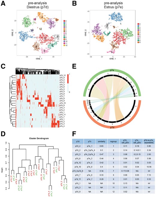
Cluster match of mammary gland epithelial cells at different phases of the estrus cycle. (A) Pre-analysis of cells from diestrus phase. (B) Pre-analysis of cells from estrus phase. (C) Heat map of the hierarchical clustering of subgroups by the existence of marker genes. Each column is a marker gene for one of the subgroups. (D) Dendrogram of the hierarchical clustering. (E) Circos plot of the matched subgroups. The 13 black sectors highlighted by the red sector represent 13 groups in diestrus as in Figure 3A, while the 10 sectors highlighted by the green sector represent 10 groups in estrus as in Figure 3B. The width of the black sectors represents the percentage of cells in each sample. Matched groups are linked by chord, and the transparency represents the similarity of the matched groups, with less transparency indicating more similar. (F) ClusterMap results for the quantification of the sample comparisons

Fig. 4.

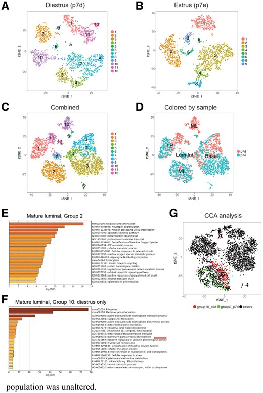
Regrouping of mammary gland epithelial cells. (A) Re-colored t-SNE plot based on matching results for diestrus phase. (B) Re-colored t-SNE plot based on matching results for estrus phase. (C) Re-colored t-SNE plot based on matching results for the combined dataset. Matched groups were recolored in the same color and with the same label through all three t-SNE plots. (D) t-SNE plot with cells colored by sample. (E and F). Gene ontology and pathway analysis for the new marker genes of Regroup 2 and 10 in the combined sample (C) using Metascape. (G) t-SNE plot of CCA analysis. Cells of Regroup 2 and 10 in diestrus, defined as in Figure 4A are highlighted in green and red

In this case, there are three types of matching sub-groups: one-to-one, one-to-multiple, and singleton. For example, Regroup 1 matched p7d_4 and p7e_1, which are tightly clustered together in the combined sample (Fig. 4D). Regroup 2 and 3 matched more than one sub-group from the estrus sample to a single group in the diestrus sample. For both cases, we can see cells in these two sub-groups (p7e_3 and p7e_4, p7e_0 and p7e_2) in estrus are closely related and adjacent to each other (Fig. 3B). Regroup 7, 10 and 11 only include sub-groups from diestrus with no matching sub-groups from estrus, suggesting these sub-groups uniquely exist in diestrus.

Based on known markers (Supplementary Fig. S3A and B), we can label Regroup 2, 5, 6 and 10 as mature luminal (ML), Regroup 1, 11 and 12 as luminal progenitors (LPs), Regroup 9 as luminal intermediate (Lum Int), and Regroup 3, 4, 7 and 8 as basal cells (Fig. 4A–D). In line with Pal’s observations, we note that the basal population increases slightly in estrus (43–47%), ML becomes two major sub-types (Regroup 2 and 10) and the Lum Int is substantially reduced (5–1%) in the diestrus phase. However, ClusterMap unveils more detailed changes between diestrus and estrus that were not identified previously. We found that in basal, Regroup 3 was increased substantially in estrus (8–35%) with large separability (2.93), whereas Regroup 7 is missing in estrus (Figs 3F and 4A–D). Also, Regroup 8 in basal is substantially altered between the two phases with a separability of 7.13. In the ML population, we noticed that although both Regroup 2 and 10 are ML, Regroup 2 in diestrus resembles ML in estrus more closely than Regroup 10 (Fig. 3D and F). Although cells in Regroup 2 are a mixture of both phases, cells in Regroup 10 are exclusively from the diestrus phase (Fig. 4C and D). These suggest that a subset of ML cells in diestrus begin to diverge, but ML cells in estrus are more homogenous. Pal et al. also observed that one of the ML subtypes was tightly associated with ML signature genes such as PgR, but they neglected to identify that there were different relationships between the two ML subtypes in diestrus and the ML in estrus. One of the ML subtypes in diestrus is much closer to the ML in estrus. For the LP population (Regroup 1, 11 and 12), our analysis suggests Regroups 11 and 12 are unique sub-types in diestrus (Fig. 4A–D), while Pal et al.’s analysis concluded that the LP population was unaltered.

We further characterized the unique groups (7, 10 and 11) in the diestrus phase through gene ontology and pathway analysis (Tripathi et al., 2015). We found that the marker genes of these groups were extremely enriched for the terms of ribosome biogenesis, oxidative phosphorylation and metabolic process of ribonucleotides (Fig. 4E and F, Supplementary Fig. S3C and D). These findings reflect the increased levels of progesterone in diestrus, which functions as a potent mitogen to stimulate expansion of mammary epithelia at this stage. Only some subpopulations of basal, ML and LP in diestrus responded to progesterone to undergo rapid cell cycle progression, potentially suggesting the existence of differential regulation of mitogen-related cell signaling among sub-populations of the same cell type. Intriguingly, we noted Regroup 10 cells in diestrus are associated with the development of mammary gland alveoli, indicating that some of the cells within this group possess trans-differentiation potential for alveolar development (Fig. 4F, Visvader, 2009). In addition, we observed a drastic increase in the number of Regroup 3 cells with characteristics of smooth muscle in estrus, indicating there may be a contractile switch of myoepithelial cells for lactation preparation during this period (Supplementary Fig. S3D, Sopel, 2010).

For comparison with ClusterMap, we also performed CCA (Butler et al., 2018, Fig. 4G and Supplementary Fig. S4A–D) and scmap (Kiselev et al., 2018, Supplementary Fig. S4E and F) on the epithelial cell datasets. In the CCA analysis, the two samples mixed more evenly under canonical correlation vector space (Supplementary Fig. S4B). Note that the two separated groups, Regroup 2 and 10 (Fig. 4A) of ML (marked by Prlr) in diestrus were not separated into sub-groups after the CCA analysis (Fig. 4G and Supplementary Fig. S4A and B). This indicated that CCA reduced the difference between sub-groups even in the same sample, which led to existing sub-groups becoming less distinguishable. Butler et al. (2018) observed this effect as well for rare populations and suggested using PCA for further analysis. However, the sub-group 10 in the diestrus phase (Fig. 4A and C) was not a rare population. With CCA only, we may miss the detection of these sample specific sub-groups identified by ClusterMap. Thus, CCA and ClusterMap provide different views of comparing multiple scRNA-Seq datasets. In the scmap, we first mapped cells in estrus to the sub-groups of diestrus. With stringent threshold 0.7, it shows largely unassigned cells (Supplementary Fig. S4E, right). After we loosed the threshold to 0.5 (Supplementary Fig. S4E, left), the results is much more similar to ClusterMap, which confirmed our matching results again. However, when we mapped cells in diestrus back to estrus, some results of scmap become confused. There are very few cells in p7e_3 mapped to p7d_1 (Supplementary Fig. S4E), but many cells in p7d_1 are mapped to p7e_3 (Supplementary Fig. S4F, purple dots). Another example, while cells in p7d_0 are mapped to both p7e_2 and p7e_6, but p7e_2 are mapped to p7d_5 and p7e_6 are mapped to p7d_7, p7d_8, nothing to p7d_0. Taken together, scmap can provide higher resolution of sample matching, but might have difficulty to coordinate the results across multiple samples.

3.2 Peripheral blood mononuclear cells under immune stimulus

We next applied ClusterMap to compare effects of experimental treatments on each cellular population. The datasets we used were generated in the study of Kang et al. (2018). Peripheral blood mononuclear cells (PBMCs) from each of eight patients were either untreated as a control or activated with recombinant interferon-beta (IFN-β) for 6 h. The same number of IFN-β-treated and control cells from each patient was pooled and subjected to single-cell sequencing on a 10× Chromium instrument. Transcriptomes of 14 619 control and 14 446 IFN-β-treated single cells were obtained.

The pre-analysis defined 11 and 13 sub-groups for the control and stimulated conditions respectively (Supplementary Fig. S5A). With hierarchical clustering and the purity tree cut approach (Supplementary Fig. 5A and B), ClusterMap matched most sub-groups, except the Regroups 10, 11 and 12 (Fig. 5C, Supplementary Fig. S5B). We confirmed that the matched groups expressed the same known marker genes, demonstrating that matching worked correctly (Supplementary Fig. S5E and F). There is no obvious change in the percentage of each cell type after stimulation, which is consistent with Kang et al.’s conclusion. For Regroup 10 and 12, although both groups express some megakaryocyte marker genes, such as PPBP (Supplementary Fig. S5E and F), other marker genes of Regroup 10 and 12 do not overlap with each other very well, placing them in distantly related clusters (Fig. 5A, arrows). Thus, ClusterMap considered these two sub-groups to be distinct new groups. However, Regroup 10 and 12 partially overlap in the combined analysis (Fig. 5D). We suspect that this inconsistency might be due to the relatively small population size in both sub-groups. The small population size increases the false positive rate of identified marker genes, which negatively affects the performance of ClusterMap.

Fig. 5.

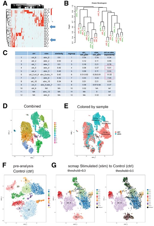
ClusterMap analysis of PBMCs datasets with immune stimulation. (A) Heat map of marker genes. (B) Dendrogram of the hierarchical clustering of marker genes. (C) Quantitative comparison of the sub-groups between samples by ClusterMap. (D) Re-colored t-SNE plot based on matching results for the combined dataset. (E) t-SNE plot with cells colored by sample. (F) Pre-analysis of the control condition. (G). scamp results of mapping stimulated condition to control at threshold 0.3 and 0.5. Cells are colored the same as their assigned sub-groups in (F)

Based on known marker genes, we assigned new Group 1, 2, 3 to CD4+ T cells, Group 5 to B cells, Group 6 to CD14+CD16– monocytes, Group 4 to CD14+CD16+ monocytes, Group 7 and 8 to dendritic cells (DCs), Group 10 and 12 to megakaryocytes, Group 11 to erythroblast and Group 9 to a mixture of natural killer cells and CD8+ T cells (Supplementary Fig. S5E and F). We observe a wide range of separability measures across matched sub-clusters, indicating the different sub-groups responds to IFN-β stimulation very differently. For instance, the Regroup 1, 2, 3 and 9 of T cells and NK cells was less affected, while the IFN-β stimulation affected monocytes and DCs (Regroup 4, 6 and 7) much more than the other immune cells (Fig. 5C red-dashed boxes, D and E). This is confirmed in the t-SNE plot from the combined analysis, the distance of cells from the two conditions in Regroup 4, 6 and 7 are much farther than the other groups (Fig. 5D and E). In addition, we note that although Regroup 5 and 6 match with comparable similarity (0.48 and 0.45), the separability of the two groups is quite different (0.55 and 11.03) (Fig. 5C). This suggests that the overlapping of marker genes is similar for the two regroups, but the changes in transcriptome expression levels may be drastically different.

Butler et al. (2018) applied CCA to analyze the same immune stimulated dataset. By aligning each cell, the samples are scaled to become as similar as possible. The global differences in the original datasets were treated as a batch effect instead of biological effect. However, the IFN-β stimulus was expected to trigger a widespread immune response of PBMCs (Kang et al., 2018). It is hard to determine if the effect is due to actual biological treatment or technical issues. Additionally, we observed DCs (Regroup 7) and monocytes (Regroup 4 and 6) respond to IFN-β the most (Fig. 5D and E), while Butler et al. observed plasmacytoid DC respond to the stimulus the most, but did not see an obvious response for the myeloid and lymphoid cells.

We also performed scmap analysis for comparison with ClusterMap. We mapped the stimulated condition to the control first (Fig. 5F and G). We had to decrease the threshold to 0.3 to reduce the number of unassigned cells due to the existence of global effect (Fig. 5G). Most of the matches are the same as the results in ClusterMap, except for the CD14+ monocytes. Scmap assign stim_0 to ctrl_8 instead of ctrl_0 (Fig. 5G and Supplementary Fig. S5A). This is due to the stimulation affecting the CD14+ monocytes the most (Fig. 5D and E) and shifting the group stim_0 towards the centroid of ctrl_8. By using the absolute expression level of the centroid of cells, scmap did not capture the relative structure of the sub-groups within one sample. In other words, although CD14+ monocytes were affected dramatically under stimulation, the molecular features of CD14+ monocytes still identify them as CD14+ monocytes when compared with other sub-groups in the same condition. ClusterMap was able to use this relative information to match the sub-types correctly.

3.3 PBMCs replicates and negative controls

To determine if our method introduced any spurious matches, we used ClusterMap to compare (i) two replicated datasets, (ii) datasets from totally different tissues and (iii) datasets with no shared marker genes at all. Ideally, clusters in replicated data should match each other in a one-to-one manner with minimal differences observed as a true positive control. The 4K and 8K PBMC datasets were downloaded from the 10× Genomics public datasets (https://support.10xgenomics.com/single-cell-gene-expression/datasets/). They are PBMCs from the same healthy donor. The two datasets are replicates with different cell numbers examined, each contains about 4000 and 8000 cells, respectively.

The group matching results demonstrate that the sub-groups in the 4K PBMCs match with the 8K PBMCs in a one-to-one manner (Supplementary Figs S6 and S7). The similarity values between matched groups are also much higher than in the previous two datasets in the Sections 3.1 and 3.2 (Supplementary Fig. S6F). The chord color in the Circos plot is hence much darker (Supplementary Fig. S6E). The majority of the cell percentages of sub-groups are not changed. The separability values demonstrate that there are no obvious differences between the two samples in any of the matched pairs (Supplementary Fig. S6F). This matches the original expectation as 4K and 8K PBMCs are replicates.

Next, we downloaded a dataset of brain tissue from 10× Genomics public datasets (https://support.10xgenomics.com/single-cell-gene-expression/datasets/2.1.0/neurons_2000). This dataset contains 2022 cells of a combined cortex, hippocampus and sub ventricular zone of an E18 mouse. Pre-analysis clustered the cells into 8 sub-groups of different types of neurons (Supplementary Fig. S8A). We tried to match this dataset to the estrus phase of epithelial cells as shown in Section 3.1 (Supplementary Fig. S8B). Only 8.6% of total marker genes were overlapped between the two datasets. We found most of the sub-groups from the same tissue clustered together. Several sub-groups matched between tissues with very low similarity (0.08, 0.04, Supplementary Fig. S8C), which should be considered as unmatched groups. As an additional check, we removed the overlapping genes between the two datasets from the marker gene list of the estrus sample (12.1%) to generate an artificially mutually exclusive dataset. As a result, the two datasets clustered totally independently (Supplementary Fig. S8D). In this case, ClusterMap will return nothing and suggest no matched groups. Together, these three cases show that ClusterMap will not find spurious relationships where they do not exist in the data. In summary, we demonstrated the sensitivity and the specificity of ClusterMap using both positive and negative datasets.

3.4 Smart-seq2 dataset

To test the scope of our method, we also applied ClusterMap to a Smart-seq2 dataset. The dataset contains different sub-types of T cells from 12 patients (Zhang et al., 2018). The number of cells in each patient range from 210 to 1253. The cell sub-types are pre-defined in the original study. We tried to match the pre-defined sub-types (Supplementary Fig. S9B) across patients to test whether our method can match the sub-types correctly. To simplify the comparison, we kept the sub-types of CD4 and CD8 T cells only and the sub-types with more than 20 cells in a patient. Marker genes were filtered by False Discovery Rate (FDR) < 0.05. The results of 12 patients are shown in Supplementary Figure S2C and Supplementary Table S1. We also took two patients out as an example, and compare the two samples (Supplementary Fig. S9A and C). ClusterMap performed well on both 12 and 2 samples, matching most of the corresponding sub-types correctly. Compare to 10x genomics datasets, Smart-seq2 datasets tend to contain much smaller number of cells, and are less powerful for defining sub-groups and enriched marker genes for each group. As long as the marker genes can be defined confidently, ClusterMap processes it the same as 10× datasets.

4 Discussion

Although CCA analysis is convenient to merge multiple samples for comparison, it may ignore the confounding of batch and biological effect and shrink the difference between sub-groups. Scmap is useful for mapping a new dataset to known reference datasets, but may be not easy for the comparison across multiple samples from different conditions. In addition, its performance may be affected by large global effects. Using marker genes and purity tree cut, ClusterMap match multiple samples reliably at cluster level and overcomes batch effects directly. There is no need to remove batch effects across samples before matching sub-groups by ClusterMap. Meanwhile, ClusterMap provides useful quantification and clear visualization as a whole workflow, which are convenient for interpretation and downstream analysis.

Due to the limitation of current scRNA-seq experimental design, batch effects and biological effects are always confounded. It is challenging to distinguish batch effect from treatment effect. During the matching step of ClusterMap, batch effects will not affect the matching results. Because marker genes for each sub-group are identified relative to the rest of the sub-groups within a given sample, matching based on the existence (binary) of marker genes will overcome the batch effect. Separability can indicate the existence of batch effects or systematic variation, if large separability values are observed over all matched groups. There are many studies on comparison of multiple scRNAseq datasets from different batches, such as the mutual nearest neighbors method (Haghverdi et al., 2018) or the distribution-matching residual networks method (Shaham et al., 2017). If necessary, separability can be applied after batch effect correction.

As a downstream analysis approach of scRNA-seq, ClusterMap relies on the pre-analyzed data. The clustering analysis of each single sample and the marker genes identified for each sub-group will affect the quality of the matching results. Refining marker gene lists will certainly improve the sub-group matching. It is important to define meaningful sub-groups for each sample first before starting a cluster comparison. The regroup step in ClusterMap refines the clustering based on the matched results, possibly merging some similar sub-groups in the same sample.

Similarity measures how well a pair matches with each other compared with other groups based on the marker genes. Separability measures how much the group properties change between paired groups. They can both reflect the relationship of the paired groups, but in different ways. Typically, as similarity rises, separability decreases. However, it is possible that a pair has similar marker genes, but separates far apart (Regroup 6 and Fig. 5C, F and G). This is due to the use of binary values of marker genes to compare between groups while absolute expression level is used to compare cell distance within paired groups.

The clustering analysis may be performed on the combined samples as well. Better resolution will be gained by the increased cell numbers of the pooled dataset. However, the new clustering results will be hard to match back to the sub-groups in each single sample. The regrouping results in ClusterMap keep the grouping information for the single samples. It also makes sense to compare the match-defined new groups and the clustering-analysis-defined new groups in the combined sample.

An R package and documentation for ClusterMap is available on GitHub (https://github.com/xgaoo/ClusterMap). The code and results for the pre-analysis of the datasets in this study are also available.

The epithelial datasets, immune stimulated datasets and the Smart-seq2 of T cells datasets were downloaded from Gene Expression Omnibus under accession numbers GSE103272, GSE96583 and GSE108989. The PBMC replicates datasets and the brain cells dataset were downloaded from the 10× Genomics support datasets website at (https://support.10xgenomics.com/single-cell-gene-expression/datasets/2.1.0/pbmc4k, https://support.10xgenomics.com/single-cell-gene-expression/datasets/2.1.0/pbmc8k and https://support.10xgenomics.com/single-cell-gene-expression/datasets/2.1.0/neurons_2000).

Funding

This work has been supported by Stowers Institute for Medical Research and CAMS Initiative for Innovative Medicine (2018-I2M-AI-010).

Conflict of Interest: none declared.