A network of networks approach for modeling interconnected brain tissue-specific networks

Abstract

Motivation

Recent sequence-based analyses have identified a lot of gene variants that may contribute to neurogenetic disorders such as autism spectrum disorder and schizophrenia. Several state-of-the-art network-based analyses have been proposed for mechanical understanding of genetic variants in neurogenetic disorders. However, these methods were mainly designed for modeling and analyzing single networks that do not interact with or depend on other networks, and thus cannot capture the properties between interdependent systems in brain-specific tissues, circuits and regions which are connected each other and affect behavior and cognitive processes.

Results

We introduce a novel and efficient framework, called a ‘Network of Networks’ approach, to infer the interconnectivity structure between multiple networks where the response and the predictor variables are topological information matrices of given networks. We also propose Graph-Oriented SParsE Learning, a new sparse structural learning algorithm for network data to identify a subset of the topological information matrices of the predictors related to the response. We demonstrate on simulated data that propose Graph-Oriented SParsE Learning outperforms existing kernel-based algorithms in terms of F-measure. On real data from human brain region-specific functional networks associated with the autism risk genes, we show that the ‘Network of Networks’ model provides insights on the autism-associated interconnectivity structure between functional interaction networks and a comprehensive understanding of the genetic basis of autism across diverse regions of the brain.

Availability and implementation

Our software is available from https://github.com/infinite-point/GOSPEL.

Supplementary information

Supplementary data are available at Bioinformatics online.

1 Introduction

Neurodevelopmental disorders are characterized by impaired functions of the central nervous system that can appear early in development and often persist into adulthood (Tollefsbol, 2017). The spectrum of developmental impairment varies and includes intellectual disabilities, communication and social interaction challenges and attention and executive function deficits (American Psychiatric Association, 2013). Prototypical examples of neurodevelopmental disorders are intellectual disability, autism spectrum disorder (ASD), epilepsy and schizophrenia (SCZ).

Recent sequence-based analyses have unraveled a complex, polygenic and pleiotropic genetic architecture of neurodevelopmental disorders, and have identified valuable catalogs of genetic variants as genetic risk factors for neurodevelopmental disorders (Gratten et al., 2014). However, it remains unknown if and how genetic variants interact with environmental and epigenetic risk factors to impart brain dysfunction or pathology.

For a mechanical understanding of specific genetic variants in neurodevelopmental disorders, integrative network approaches have attracted much attention in recent years due to their interdisciplinary applications. Several state-of-the-art network-based analyses provide an organizational framework of functional genomics and demonstrate that they will enable the investigation of relationships that span multiple levels of analysis (Gandal et al., 2018; Krishnan et al., 2016; Parikshak et al., 2013). These methods were mainly designed for modeling and analyzing single networks that do not interact with or depend on other networks. However, the brain consists of a system of multiple interacting networks and must be treated as such. In multiple interacting networks, the failure of nodes in one network generally leads to the failure of dependent nodes in other networks, which in turn may cause further damage to the first network, leading to cascading failures and catastrophic consequences (Gao et al., 2012). It is known, e.g. that different kinds of brain-specific tissues, circuits and regions are also coupled together and affect behavior and cognitive processes, and thus dysfunctions of the central nervous system in neurodevelopmental disorders have been the result of cascading failures between interdependent systems in the brain. However, no systematic mathematical framework is currently available for adequately modeling and analyzing the consequences of disruptions and failures occurring simultaneously in interdependent networks.

We address this limitation by developing a novel and efficient framework, called the ‘Network of Networks’ (NoN) approach, that will provide useful insights on the properties and topological structure of the inter-correlations between functional interaction networks (Fig. 1). Motivated by a perspective on structural equation models, we model the topological information of each network as a weight sum of the topological information of all other networks. Our NoN model enables the exploitation of the interconnectivity structure between complex systems. It has shown to be effective in aiding the comprehensive understanding of the genetic basis of neurodevelopmental disorders across diverse tissues, circuits and regions of the brain.

Fig. 1.

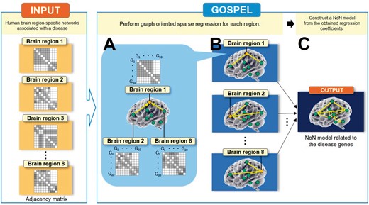
Overview of GOSPEL, an example for the case where $n=10,p=8$⁠. Assume that we are given the human brain region-specific networks associated with a disease. As input, GOSPEL requires p adjacency matrices generated from p networks with n nodes, where n and p indicate the number of nodes (genes) and features (brain regions), respectively. Block ‘A’ shows that GOSPEL estimates the brain regions which are related to ‘Brain region 1’ by performing a graph-oriented sparse regression. In this example, ‘Brain region 2’ and ‘Brain region 8’ are related to ‘Brain region 1’. Block ‘B’ illustrates that a regression is performed on each of the brain regions. As with block ‘A’, block ‘B’ estimates the relationship between the target brain region and the other brain regions. Block ‘C’ expresses that the output of GOSPEL, the ‘Network of Networks’ model related to the disease genes, is constructed from the obtained regression coefficients

Our main contributions are summarized as follows:

1. We define a statistical framework of structural equation models for inferring the interconnectivity structure between multiple networks where the response and the predictor variables are given networks which have topological information. Structural equation modeling is a statistical method used to test the relationships between observed and latent variables (Civelek, 2018). We extend the structural equation models for modeling the effects of network–network interactions.

2. In order to accomplish this, we propose a sparse learning algorithm for network data, called Graph-Oriented SParcE Learning (GOSPEL), to find a subset of the topological information matrices of the predictor variables (networks) related to the response variable (network). More specifically, we propose to use particular forms of diffusion kernel-based centered kernel alignment (Cortes et al., 2012) as a measure of statistical correlation between graph Laplacian matrices, and solve the optimization problem with a novel graph-guided generalized fused lasso. This new formulation allows the identification of all types of correlations, including non-monotone and non-linear relationships, between two topological information matrices.

3. We use a Bayesian optimization-based approach to optimize the tuning parameters of the graph-guided generalized fused lasso and automatically find the best fitting NoN model with an acquisition function. The software package that implements the proposed method in the R environment is available from https://github.com/infinite-point/GOSPEL.

We describe our proposed framework and algorithm, and discuss properties in Section 2. Section 3.1 contains a simulation study which demonstrates the performance of the proposed method. We use human brain-specific functional interaction networks and known risk genes with strong prior genetic evidence of ASD and identify the interconnectivity between these networks in Section 3.2. Section 4 provides concluding remarks.

2 Materials and methods

Our goal is to infer the interconnectivity structure between multiple networks from topological information matrices of given networks. To do this, we make the assumption that each topological information matrix for a given network can be expressed by the linear combination of the topological information matrices of the other given networks. Sparse regression is performed on each of the given networks in order to identify a subset of the topological information matrices of the predictors related to the response. After this computation, NoN model is constructed from the obtained regression coefficients. In this section, we first explain the problem setting, and then present our method, GOSPEL.

2.1 Problem setting

Suppose that we are given p undirected networks consisting of n vertices (nodes) $V^{(i)}=\{v_1^{(i)},\dots ,v_n^{(i)}\}\hspace{0.17em}(i=1,\dots ,p)$ linked by edges. The i-th adjacency matrix ${\mathit{A}}^{(i)}\in {\mathbb{R}}^{n\times n}$ associated with the i-th undirected network is defined as

$$A_{j,k}^{(i)}=\{\begin{array}{cc}{w}_{j,k}^{(i)}\hfill & \hspace{0.17em}\text{if}\hspace{0.17em}j\ne k\hspace{0.17em}\text{and}\hspace{0.17em}{v}_j^{(i)}\hspace{0.17em}\text{links}\hspace{0.17em}\text{with}\hspace{0.17em}{v}_k^{(i)},\hfill \\ 0\hfill & \hspace{0.17em}\text{otherwise},\hfill \end{array}$$

where $w_{j,k}^{(i)}\in [0,1]$ denotes the probability of connectivity between $v_j^{(i)}$ and $v_k^{(i)}$ in the i-th network. Here, we compute graph Laplacian matrix ${\mathit{L}}^{(i)}$⁠:

$$L_{j,k}^{(i)}=\{\begin{array}{cc}\text{deg}\left(v_j^{(i)}\right)\hfill & \hspace{0.17em}\text{if}\hspace{0.17em}\mathit{j}=\mathit{k},\hfill \\ -w_{j,k}^{(i)}\hfill & \hspace{0.17em}\text{if}\hspace{0.17em}\mathit{j}\ne \mathit{k}\hspace{0.17em}\text{and}\hspace{0.17em}{\mathit{v}}_{\mathit{j}}^{(\mathit{i})}\hspace{0.17em}\text{links}\hspace{0.17em}\text{with}\hspace{0.17em}{\mathit{v}}_{\mathit{k}}^{(\mathit{i})},\hfill \\ 0\hfill & \hspace{0.17em}\text{otherwise},\hfill \end{array}$$

where $\text{deg}\left(v_j^{(i)}\right)$ denotes the weighted degree of $v_j^{(i)}$⁠, the sum of the j-th row of ${\mathit{A}}^{(i)}$⁠. Then let us kernelize the graph Laplacian matrix. Let ${\mathit{K}}^{(i)}$ be the diffusion kernel matrix for ${\mathit{L}}^{(i)}$⁠:

$${\mathit{K}}^{(i)}=\text{exp}\hspace{0.17em}\{-{\mathit{L}}^{(i)}/{\gamma }^{(i)}\},$$

where ${\gamma }^{(i)}$ is a kernel parameter. This kernel matrix is centered and normalized as follows:

$${\overline{\mathit{K}}}^{(i)}=\mathit{H}{\mathit{K}}^{(i)}\mathit{H},$$

$${\tilde{\mathit{K}}}^{(i)}={\overline{\mathit{K}}}^{(i)}/\left|\right|{\overline{\mathit{K}}}^{(i)}|{|}_F,$$

where $\left|\right|·|{|}_F$ denotes the Frobenius norm, $\mathit{H}$ indicates the centering matrix $\mathit{H}={\mathit{I}}_n-\frac{1}{n}{\mathbf{1}}_n{\mathbf{1}}_n^{\top }$⁠, ${\mathit{I}}_n$ is an n × n identity matrix, and ${\mathbf{1}}_n$ is an n-dimensional vector with all ones.

We assume that the diffusion kernel matrix of the i-th network can be represented by the linear combinations of centered and normalized diffusion kernel matrices of the other networks as follows:

$${\tilde{\mathit{K}}}^{(i)}=\sum _{j=1}^p{\beta }_j^{(i)}{\tilde{\mathit{K}}}^{(j)}+{\mathit{\epsilon }}^{(i)},$$

where $\left\{{\beta }_j^{(i)}|\hspace{0.17em}\hspace{0.17em}j=1,\dots ,p,\hspace{0.17em}\hspace{0.17em}{\beta }_i^{(i)}=0\right\}$ denotes a regression coefficient corresponding to predictor ${\tilde{\mathit{K}}}^{(j)}$ and response ${\tilde{\mathit{K}}}^{(i)}$⁠, and ${\mathit{\epsilon }}^{(i)}\in {\mathbb{R}}^{n\times n}$ is a Gaussian noise matrix whose elements follow $\mathrm{N}(0,{\sigma }_i^2)$⁠.

The estimation for the network structure of the given networks is available by applying GOSPEL to all the cases where $i=1,\dots ,p$⁠. Note that, in an ordinary regression problem for n samples and p predictors, both the predictors and the response are given as n-dimensional vectors. In our problem setting, however, they are given as n × n networks.

2.2 Graph Oriented Sparse Learning (GOSPEL)

The optimization problem of GOSPEL is as follows:

$$\begin{array}{c}\underset{{\beta }_1^{(i)},\dots ,{\beta }_p^{(i)}}{\text{min}}\left|\right|{\tilde{\mathit{K}}}^{(i)}-\sum _{j=1}^p{\beta }_j^{(i)}{\tilde{\mathit{K}}}^{(j)}|{|}_F^2+{\lambda }_1^{(i)}\sum _{j,k=1}^p{R}_{j,k}^{(i)}\hspace{0.17em}|{\beta }_j^{(i)}-{\beta }_k^{(i)}|+{\lambda }_2^{(i)}\sum _{j=1}^p|{\beta }_j^{(i)}|,\end{array}$$

(1)

where ${\lambda }_1^{(i)},{\lambda }_2^{(i)}$ are regularization parameters, and $|·|$ indicates the ${\ell }_1$ norm. ${\mathit{R}}^{(i)}\in {\mathbb{R}}^{p\times p}\hspace{0.17em}(i=1,\dots ,p)$ expresses a matrix whose elements consist of correlations between predictors, where

$$R_{j,k}^{(i)}=\{\begin{array}{cc}1\hspace{0.17em}\hspace{0.17em}\hfill & \text{if}\hspace{0.17em}|\text{CKA}({\tilde{\mathit{K}}}^{(j)},{\tilde{\mathit{K}}}^{(k)})|\ge {\tau }^{(\mathrm{i})}\hspace{0.17em}\hspace{0.17em}\text{and}\hspace{0.17em}\hspace{0.17em}j\ne k,\hfill \\ 0\hspace{0.17em}\hspace{0.17em}\hfill & \text{otherwise}.\hfill \end{array}$$

$\text{CKA}({\tilde{\mathit{K}}}^{(j)},{\tilde{\mathit{K}}}^{(k)})$ denotes a correlation between kernel matrices ${\tilde{\mathit{K}}}^{(j)}$ and ${\tilde{\mathit{K}}}^{(k)}$⁠; this measure is called the Centered Kernel Alignment (CKA) (Cortes et al., 2012), and ${\tau }^{(i)}$ indicates a threshold. CKA captures the non-linear relationship between two matrices if such a relationship exists.

The definition of CKA is as follows:

$$\text{CKA}({\tilde{\mathit{K}}}^{(j)},{\tilde{\mathit{K}}}^{(k)})={\langle {\tilde{\mathit{K}}}^{(j)},{\tilde{\mathit{K}}}^{(k)}\rangle }_F$$

where ${\langle ·,·\rangle }_F$ indicates the Frobenius inner product. The Frobenius inner product can be interpreted as an inner product of two vectorized matrices, and thus we can apply the properties of Pearson’s correlation coefficient (Sharma, 2005) to CKA. Unless the elements of ${\tilde{\mathit{K}}}^{(j)}$ or ${\tilde{\mathit{K}}}^{(k)}$ are all zero (we omit such cases in the computation of GOSPEL), this definition implies that the value of CKA becomes zero when ${\tilde{\mathit{K}}}^{(j)}$ and ${\tilde{\mathit{K}}}^{(k)}$ have no correlation and the CKA value takes ±1 when the two matrices are strongly correlated. In practice, the value of the diffusion kernel-based CKA ranges from −1 to 1 because of the positive semi-definiteness of the diffusion kernel matrix (Lafferty and Kondor, 2002).

GOSPEL optimization Equation (1) consists of the squared Frobenius norm term, the graph-guided-fused-lasso regularization term (Chen et al., 2012), and the lasso regularization term (Tibshirani, 1996). If $R_{j,k}^{(i)}$ of the graph-guided-fused-lasso regularization term is zero, the equation becomes solely dependant on the lasso regularization term. Table 1 summarizes the behavior of ${\beta }_j^{(i)}$ and ${\beta }_k^{(i)}$ in GOSPEL optimization. The table shows that GOSPEL estimates all the relevant predictor-networks to the response-network, and also eliminates irrelevant predictor-networks to the response-network. For more detail on the behavior of the regression coefficients, see Section 1 in the Supplementary Material. The sparsity of the elements of ${\mathit{\beta }}^{(i)}$ helps to facilitate the interpretation of the computation results. By extension, the interpretation of the network structure of given networks is also facilitated.

Table 1.

Behavior of ${\beta }_j^{(i)}$ and ${\beta }_k^{(i)}$ in GOSPEL optimization

Correlations		Regression coefficients
${\tilde{\mathit{K}}}^{(i)},{\tilde{\mathit{K}}}^{(j)}$	${\tilde{\mathit{K}}}^{(j)},{\tilde{\mathit{K}}}^{(k)}$	${\beta }_j^{(i)}$	${\beta }_j^{(i)},{\beta }_k^{(i)}$
Correlated	Uncorrelated	A real value except zero	—
Uncorrelated	Uncorrelated	Zero	—
Correlated	Correlated	—	Real values except zero
Uncorrelated	Correlated	—	Zeros

Note: When ${\tilde{\mathit{K}}}^{(j)}$ and ${\tilde{\mathit{K}}}^{(k)}$ are uncorrelated, i.e. $R_{j,k}^{(i)}=0$⁠, the value of ${\beta }_j^{(i)}$ is estimated depending on the correlation between response ${\tilde{\mathit{K}}}^{(i)}$ and predictor ${\tilde{\mathit{K}}}^{(j)}$⁠. Similarly, the value of ${\beta }_k^{(i)}$ is computed depending on the correlation between the response and the k-th predictor. On the other hand, when ${\tilde{\mathit{K}}}^{(j)}$ and ${\tilde{\mathit{K}}}^{(k)}$ are correlated, i.e. $R_{j,k}^{(i)}=1$⁠, ${\beta }_j^{(i)}$ and ${\beta }_k^{(i)}$ tend to take similar values depending on the correlation between the response and the i-th predictor.

Finally, we construct a NoN model utilizing the obtained regression coefficients ${\left\{{\widehat{\beta }}_j^{(i)}\right\}}_{i,j=1}^p$⁠. Let $E\subseteq \Gamma (p)\times \Gamma (p)$ be an edge set for a NoN model, where $\Gamma =\{1,\dots ,p\}$ is a node set. We employ the edge set estimation defined by Meinshausen and Bühlmann (2006):

$$E=\left\{(i,j)|\hspace{0.17em}\hspace{0.17em}{\widehat{\beta }}_j^{(i)}\ne 0\hspace{0.17em}\vee \hspace{0.17em}{\widehat{\beta }}_i^{(j)}\ne 0\right\},$$

where (i, j) indicates the pair of the i-th and the j-th nodes. Based on the graphical model $G=(\Gamma ,E)$⁠, the NoN model is constructed as the output of GOSPEL.

2.3 Computation of GOSPEL

To solve the GOSPEL optimization problem, Equation (1), we first vectorize all the kernel matrices. This produces an n²-dimensional vector associated with the response-network, and n²-dimensional vectors corresponding to p − 1 predictor-networks. This form is the same problem setting of the graph-guided generalized fused-lasso (Chen et al., 2012), G3FL, with n² samples and p − 1 features. Therefore, we employ G3FL to solve our optimization problem.

Regularization parameters ${\lambda }_1^{(i)},{\lambda }_2^{(i)}$⁠, threshold ${\tau }^{(i)}$ and kernel parameter ${\gamma }^{(i)}$ are decided by the Bayesian Optimization (Mockus, 2012). We apply the Bayesian Information Criterion (BIC) (Schwarz, 1978) as an acquisition function of the Bayesian Optimization. The BIC score for the case where the response is the i-th network is defined as

$${\text{BIC}}^{(i)}=-2{\widehat{\mathit{LL}}}^{(i)}+{\widehat{\text{df}}}^{(i)}\times \text{log}(n^2),$$

where ${\widehat{\mathit{LL}}}^{(i)}$ is the log-likelihood function:

$${\widehat{\mathit{LL}}}^{(i)}=\frac{n^2}{2}\left(\text{log}\right(\frac{2\pi }{n^2}\left|\right|{\tilde{\mathit{K}}}^{(i)}-\sum _{j=1}^p{\widehat{\beta }}_j^{(i)}{\tilde{\mathit{K}}}^{(j)}\left|{|}_F^2\right)+1),$$

and ${\widehat{\text{df}}}^{(i)}$ is the degree of freedom of the fused lasso (Tibshirani et al., 2005):

$$\begin{array}{c}{\widehat{\text{df}}}^{(i)}=p-♯\left\{{\widehat{\beta }}_j^{(i)}=0\right\}\hfill \\ -♯\left\{{\widehat{\beta }}_j^{(i)}-{\widehat{\beta }}_k^{(i)}=0\hspace{0.17em}|\hspace{0.17em}j<k,\hspace{0.17em}{\widehat{\beta }}_j^{(i)},{\widehat{\beta }}_k^{(i)}\ne 0\right\}.\hfill \end{array}$$

In the Bayesian Optimization, we select the set of parameter values which minimizes the BIC score.

3 Results

3.1 Simulations

We generate synthetic data and evaluate the performance of GOSPEL in order to gain insight into feature selection in the regression problem for network data. As synthetic data, we prepare three representative complex network models which have different structures: random networks (Erdös and Rényi, 1959), scale-free networks (Barabási and Albert, 1999) and small-world networks (Watts and Strogatz, 1998).

For each network model, 30 predictor-networks are prepared so that the first four predictors have the following linear or non-linear relationships:

$$A_{k,l}^{(j)}=\{\begin{array}{cc}{A}_{k,l}^{(1)}\hfill & j=2,\hspace{0.17em}\text{and}\hspace{0.17em}k\ne l,\hfill \\ \hspace{0.17em}\text{sin}\hspace{0.17em}\left(\pi A_{k,l}^{(1)}\right)\hfill & j=3,\hspace{0.17em}\text{and}\hspace{0.17em}k\ne l,\hfill \\ 4{\left(A_{k,l}^{(1)}-0.5\right)}^3+0.5\hfill & j=4,\hspace{0.17em}\text{and}\hspace{0.17em}k\ne l,\hfill \\ 0\hfill & j=1,\dots ,30\hspace{0.17em}\text{and}\hspace{0.17em}k=l.\hfill \end{array}$$

After this operation, we randomly shuffle 5% of the rows and columns of ${\left\{{\mathit{A}}^{(j)}\right\}}_{j=1}^4$⁠, and 100% of the rows and columns of ${\left\{{\mathit{A}}^{(j)}\right\}}_{j=5}^{30}$⁠, in order to confirm whether GOSPEL can select only the relevant (similar) predictor-networks to the response-network.

Using the four predictors, we generate the following two signal types of response-networks.

• Additive type: $\hspace{0.17em}{\mathit{A}}^{(\mathrm{i})}=\frac{1}{4}\sum _{\mathrm{j}=1}^4{\mathit{A}}^{(\mathrm{j})},$

• Non-additive type:$\hspace{0.17em}{\mathit{A}}^{(\mathrm{i})}=\frac{1}{2}\sum _{\mathrm{j}=1}^2{\mathit{A}}^{(2\mathrm{j}-1)}○{\mathit{A}}^{(2\mathrm{j})},$

where $○$ indicates the element-wise product. Figure 2 shows plot examples of these adjacency matrices. As shown in Figure 2, we set the first four predictor-networks as similar to the two types of responses, and as relevant to these responses. This setting expresses our assumption; a disease cascades along the networks which have overall topological similarity but not necessarily identical structures.

Fig. 2.

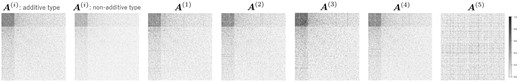
Plot example of adjacency matrices in simulation, in the case where network type is scale-free. Two plots on the left end indicate the response-networks whose signal types are additive and non-additive, respectively. ${\mathit{A}}^{(1)},\dots ,{\mathit{A}}^{(4)}$ are the predictor-networks relevant to the response-networks, and the rest 26 non-relevant predictor-networks are set like ${\mathit{A}}^{(5)}$

The diffusion kernel corresponding to the response-network is set as ${\tilde{\mathit{K}}}^{(i)}+{\mathit{\epsilon }}^{(i)}$ with a signal-to-noise ratio =1.

We run the simulations 100 times for each combination of the network model and the signal type, varying the number of vertices as $n=\{500,1000,2000\}$⁠. We compare GOSPEL to Hilbert-Schmidt Independence Criterion Lasso (HSIC Lasso) (Yamada et al., 2014), one of the feature selection methods by the feature-wise kernelized lasso. We note that HSIC Lasso is not designed for network data and cannot be directly applied. In these simulations, HSIC lasso is applied to the centered and normalized kernel matrices as follows:

$${\displaystyle \underset{{\mathit{\alpha }}^{(\mathit{i})}}{\text{min}}}\left|\right|{\tilde{\mathit{K}}}^{(i)}-\sum _{j=1}^p{\alpha }_j^{(i)}{\tilde{\mathit{K}}}^{(j)}|{|}_F^2+\lambda \sum _{j=1}^p|{\alpha }_j^{(i)}|,$$

(2)

where $\left\{{\alpha }_j^{(i)}|\hspace{0.17em}\hspace{0.17em}i,j=1,\dots ,p,\hspace{0.17em}\hspace{0.17em}{\alpha }_i^{(i)}=0\right\}$⁠.

To assess each method’s ability to obtain true fractions of predictors related to the response, we compare true predictors to the predictors with non-zero coefficients estimated by GOSPEL and HSIC Lasso. The results were analyzed for F-measure. Table 2 shows the F-measures calculated for the 18 different settings with varying sample size and network types. The results highlight the efficacy of the graph-guided fused-lasso regularization.

Table 2.

The F-measure of the simulations

		Network model
		Random		Scale-free		Small-world
n	Signal type	GOSPEL	HSIC Lasso	GOSPEL	HSIC Lasso	GOSPEL	HSIC Lasso
500	Additive	1.000	0.273	1.000	0.964	1.000	0.238
		(0.000)	(0.149)	(0.000)	(0.069)	(0.000)	(0.008)
	Non-additive	0.999	0.288	1.000	0.235	1.000	0.256
		(0.014)	(0.161)	(0.000)	(0.001)	(0.000)	(0.047)
1000	Additive	1.000	0.276	1.000	1.000	1.000	0.248
		(0.000)	(0.168)	(0.000)	(0.000)	(0.000)	(0.082)
	Non-additive	1.000	0.246	1.000	0.235	1.000	0.251
		(0.000)	(0.078)	(0.000)	(0.000)	(0.000)	(0.109)
2000	Additive	1.000	0.244	1.000	1.000	1.000	0.243
		(0.000)	(0.077)	(0.000)	(0.000)	(0.000)	(0.076)
	Non-additive	1.000	0.245	1.000	0.241	1.000	0.235
		(0.000)	(0.079)	(0.000)	(0.057)	(0.000)	(0.001)

Note: $(·)$ denotes the standard deviation of the F-measure. The predictor-networks are generated according to the representative three network models. n indicates the number of vertices, and the response-network is generated based on the signal type. ‘HSIC Lasso’ does not mean the original one but the variant one.

We can particularly see the importance of graph-guided fused-lasso regularization when we compare GOSPEL with the similar HSIC Lasso, which does not use graph-guided fused-lasso regularization. GOSPEL succeeds in all sample sizes, network types and signal types. On the other hand, HSIC Lasso performs poorly except in the cases of additive scale-free networks. As shown in Figure 2, scale-free networks have a clear structure, and the response-networks for additive and non-additive cases, are both similar to ${\left\{{\mathit{A}}^{(j)}\right\}}_{j=1}^4$⁠. Since the additive cases may be easy to solve, HSIC Lasso works perfectly. However, regardless of the visually easy settings, HSIC Lasso fails in the non-additive cases.

It appears that the success of GOSPEL in all settings can be attributed to the graph-guided fused-lasso regularization. The graph-guided fused-lasso regularization term of GOSPEL, the second terms of Equation (1), helps to select the predictors which have similar structures to the response, by introducing the correlations between predictors into the optimization problem. The failed HSIC Lasso, on the other hand, does not use information on the correlations between predictors, and attempts to express the response through summation of the predictors alone. This operation of HSIC Lasso without the graph-guided fused-lasso regularization results in selecting non-relevant (dissimilar) predictors, and leads failures.

3.2 Real data

3.2.1 Analysis of a network of networks related to the ASD risk genes

ASD is a complex neurodevelopmental disorder driven by a multitude of genetic variants across the genome that appear as a range of developmental and functional perturbations, often in specific tissues and cell types (Vorstman et al., 2017). To construct human brain region-specific networks associated with the ASD risk genes, we adopt a manner of data construction introduced in recent studies (Duda et al., 2018; Krishnan et al., 2016). We use 17 human brain region-specific functional interaction networks (Greene et al., 2015) and 1030 known risk genes with strong genetic evidence of ASD association annotated in the Human Gene Mutation Database Professional 2017.1 (http://hgmd.cf.ac.uk/) to evaluate our proposed method. The purpose of our analysis is to investigate how the ASD risk genes may be coupled in each of the brain region-specific networks and what interconnectivity structure between these networks can be formed.

The 17 human brain regions are taken from the whole brain: the frontal lobe (the cerebral cortex), the occipital lobe (the cerebral cortex), the parietal lobe (the cerebral cortex), the temporal lobe (the cerebral cortex), the amygdala (the limbic system), the dentate gyrus (the limbic system), the hippocampus (the limbic system), the caudate nucleus (the basal ganglia), the caudate putamen (the basal ganglia), the subthalamic nucleus (the basal ganglia), the substantia nigra (the basal ganglia), the thalamus (the diencephalon), the hypothalamus (the diencephalon), the cerebellar cortex (the cerebellum), the hypophysis (the cerebellum), the nucleus accumbens (the brain ventricle) and the pons (the brain stem).

These 17 human brain region-specific functional interaction networks are built by integrating thousands of gene expressions, protein–protein interactions, and regulatory-sequence data sets using a regularized Bayesian integration approach (Greene et al., 2015). Once built, they are used as reference networks in our analysis. This network information can be downloaded from the Genome-scale Integrated Analysis of gene Networks in Tissues web site (http://giant.princeton.edu/).

We first calculate local enrichment scores for the ASD risk genes across all nodes (25 825 genes) in the network by using the Spatial Analysis of Functional Enrichment algorithm (Baryshnikova, 2016), which measures the proximity of the ASD risk genes in the neighborhood of each node. Next, in order to reconstruct the 17 human brain region-specific networks associated with the ASD risk genes, 4756 genes with highly significant local enrichment scores for the ASD risk genes (P-value <0.001) in any of the 17 networks are selected as the nodes, and the interactions between these genes are given. We apply GOSPEL to the 4756 × 4756 adjacency matrices of the 17 brain-specific regions and construct the NoN model related to the ASD risk genes.

Figure 3 shows a NoN model related to the ASD risk genes. It illustrates the relation between the functional networks of the subregions. In Figure 3, we can observe how the gene co-expression patterns related to ASD propagate across the brain. In other words, our NoN model suggests how ASD cascades through the brain.

One may assume that measuring every pair of subregion networks is enough for this estimation. To demonstrate the necessity of GOSPEL, we compare the result of the pair measurements with the NoN model, which proves that GOSPEL correctly and automatically tunes the parameters. For details, see Section 2.1 in the Supplementary Material.

Below, we evaluate the resulting model both quantitatively and qualitatively.

Fig. 3.

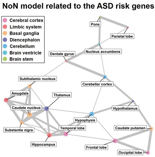
The NoN model related to the ASD risk genes. The size of the node expresses the mean value of the enrichment score associated with the brain subregion (node). The smallest, middle and the largest sized nodes express below the 30-th percentile, between the 30-th and the 60-th percentiles, and above the 60-th percentile of the enrichment score, respectively. The color of the node indicates the categorization of brain function as determined by BTO. The thickness of the edge denotes the strength of the relation between two brain subregions. The thinnest, middle and the thickest edges express the 70-th–80-th percentiles, the 80-th–90-th percentiles and above the 90-th percentile of the whole coefficients obtained by performing GOSPEL, respectively. For details, see Supplementary Table S2

(i) Quantitative interpretation of the result

For the quantitative interpretation of the resulting model, we adopt the categorization of brain function from BRENDA Tissue Ontology (BTO) (http://purl.bioontology.org/ontology/BTO), and the 3-dimensional coordinates of subregions from Talairach coordinates (TC) in the Brede Database (http://hendrix.imm.dtu.dk/services/jerne/brede/brede.html). We create the networks from BTO and TC, and compare these with our result.

Figure 4 denotes the networks generated from BTO, TC and GOSPEL. The network for BTO expresses that the subregions in the same function category link together. For more detail, see Supplementary Figure S2. The network for TC expresses that the subregions physically located near each other are linked. Note that the subregions are displayed by category from the outer part moving in to the deep part of the brain. The color and ID associated with each subregion is described in Table 3.

Fig. 4.

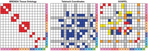
Networks created from BTO, TC and the NoN model (GOSPEL). The left image shows a network created from BTO. Up to three vertices connected along the shortest-path from the origin are linked and colored red. The center image is a network created from TC. The distances below the 35-th percentile of the Euclidean distances between two vertices (subregions) are linked and colored blue. The gray rows and columns are the subregions with no available TC. For the subregions with two coordinates (the left side and right side), we adopt the ‘Mean coordinate with ignored left/right’ according to the Brede Database. The right image is a network constructed from GOSPEL. To create this network, we ignored the links associated with the pons, the parietal lobe, the nucleus accumbens, the dentate gyrus and the hypothalamus. Since these subregions’ enrichment scores in Table 3 are low, we regarded them as not related to ASD. The red cells and the blue cells in the right image are the links which match BTO and TC, respectively. This suggests a moderate level of agreement with BTO and TC. The yellow and the orange cells are the unique links obtained by GOSPEL. The white cells in all the networks indicate ‘no link’

Table 3.

Information on the 17 subregions

ID	Subregion	Enrich.score	Com.ID
4	Temporal lobe	10.322	A
7	Hippocampus	10.320	A
15	Hypophysis	10.261	A
8	Caudate nucleus	9.890	A
12	Thalamus	9.386	A
5	Amygdala	9.259	A
11	Substantia nigra	7.967	A
10	Subthalamic nucleus	7.955	A
1	Frontal lobe	8.130	B
2	Occipital lobe	7.212	B
9	Caudate putamen	5.476	B
14	Cerebeller cortex	5.402	C
6	Dentate gyrus	3.879	C
13	Hypothalamus	3.485	C
16	Nucleus accumbens	3.290	C
17	Pons	2.849	C
3	Parietal lobe	1.318	C

Note: ‘Enrich.score’ denotes the mean value of the enrichment score. ‘Com.ID’ indicates the community ID given by the community extraction.

In Figure 4, the network of GOSPEL shows that the links in the resulting model are common with BTO in the cerebral cortex and the basal ganglia. This is expected since the Genome-scale Integrated Analysis of gene Networks in Tissues data which we used in this experiment adopts the hierarchical structure determined by BTO in the process of data construction. On the other hand, it is surprising that the links in GOSPEL are common with TC between the limbic system, the basal ganglia and the diencephalon, even though we did not consider locational information in this experiment. Table 4 indicates the consistency of links in BTO, TC and the NoN model. This table actually shows that the NoN model is similar to both BTO and TC with around $70\%$ consistency.

Table 4.

Link consistency between BTO, TC and the NoN model

	#Regions	TP	FP	TN	FN	Consistency
BTO	17	6	20	98	12	0.765
TC	14	7	10	53	21	0.659

Note: TP, FP, TN and FN are true positive, false positive, true negative and false negative, respectively.

There are 14 unique links obtained by GOSPEL. Half of these exist between the cerebral cortex and the other subregions. This is a main feature of our result. For the observation, let us imagine that the graphs for BTO and TC (the left and the center images in Fig. 4) are overlapped. One can find that there are no links between the cerebral cortex and the other regions, except for the links between the temporal lobe and the hippocampus. This is because the distances between the cerebral cortex and the other regions are far apart, since the cerebral cortex is locate in the outermost part of the brain while the other regions are locate close together in the deep part of the brain (see TC network in Fig. 4). Therefore, it is significant that half of the unique links derived from the NoN model appeared between the outer part of the brain and the deep part.

(ii) Qualitative interpretation of the result

For the qualitative interpretation of the resulting model, we investigate the NoN model in two different ways; one is by examining the structure of the NoN model, and the other is by comparing our result with the 16 abnormal functional connections identified in Yahata et al. (2016) using functional magnetic resonance imaging.

To simplify the structure of our model, first we performed a community extraction method based on random walks (Pons and Latapy, 2006). Table 3 indicates the mean value of the enrichment score and the community ID for each subregion. It also divides the resulting model into three communities according to the results of the community extraction. Let us inspect each group.

Group A is grouped around the amygdala and the thalamus. Group B is small, however, it has the interesting feature that two out of the three subregions belong to cerebral cortex. Group C consists of subregions which have low enrichment sores, and thus we consider this group as not relating to ASD and ignore it in our results.

Let us observe groups A and B in detail. In group A, the amygdala has the largest number of the thickest edges. This indicates that the gene co-expression patterns of the amygdala are reflected in the gene co-expression patterns of all the other regions within the group. As shown in Table 5, the amygdala has largely been the focus of ASD research. However, our model suggests a need to look at the relation between the other subregions and the amygdala instead of the amygdala alone.

Table 5.

Samples of the evidence for a single brain subregion associated with ASD, and consistency between our resulting model and the abnormal functional connections in Table 1 of Yahata et al. (2016)

Com.ID	Subregion	Consistency	Samples of the evidence for a single brain subregion
A	Temporal lobe	◯	Zilbovicius et al. (2000); Lee et al. (2007); Neeley et al. (2007)
	Hippocampus	△	Schumann et al. (2004); Endo et al. (2007); Conturo et al. (2008)
	Hypophysis		Iwata et al. (2011); Ćurin et al. (2003)
	Caudate nucleus	$◯$	Silk et al. (2006); Turner et al. (2006); Voelbel et al. (2006); Langen et al. (2007)
	Thalamus		Tsatsanis et al. (2003); Hardan et al. (2006); Hardan et al. (2008); Tamura et al. (2010)
	Amygdala	$◯$	Schumann et al. (2004); Schumann and Amaral (2006); Endo et al. (2007); Conturo et al. (2008);
			Schumann et al. (2009); Kleinhans et al. (2010); Nordahl et al. (2012); Kliemann et al. (2012)
	Substantia nigra		Caria et al. (2011)
	Subthalamic nucleus		Rojas et al. (2014)
B	Frontal lobe	◯◯△	Hardan et al. (2004); Schmitz et al. (2007); Scott-Van Zeeland et al. (2010); Jeong et al. (2011)
	Occipital lobe	◯	Hardan et al. (2009)
	Caudate putamen		Kumra et al. (2000)

Note: ‘$◯$’ and ‘$△$’ denote a direct and a proximate connection, respectively.

Table 6.

Link consistency between the NoN models of the three brain diseases

	ASD and SCZ	ASD and ND	SCZ and ND
Consistency	0.809	0.544	0.632

While the amygdala may be thought of as the center of functional abnormality within the brain, it is closely connected to the thalamus that is known to act as an information relay station (hub) between the subcortical areas and the cerebral cortex (Gazzaniga et al., 2009). This suggests that if there is a problem in the amygdala, the problem will not only be reflected in the other subregions in Group A, but the problem will be relayed to other parts of the brain via the thalamus.

Group B is constructed of the subregions related to the cerebral cortex. Table 5 shows that the most prominently studied subregion in this group in ASD research is the frontal lobe. Although the caudate putamen does not belong to the cerebral cortex, it may regulate threshold potential in the brain by measuring the whole activity of cerebral cortex in order to prevent explosive activation of the brain’s excitatory synapses (Braitenberg, 1986).

GOSPEL suggests that ASD cascades not only within groups A and B, but also between them from the temporal lobe or the hypophysis.

The next step is to confirm the validity of our model against the results of other accepted studies. To classify the differences between ASD and typically developed persons, Yahata et al. (2016) identified 16 abnormal functional connections using functional magnetic resonance imaging. In order to compare consistency with the results of Yahata et al. (2016), we first investigate the common subregions used in both Yahata et al. (2016) and our experiment. While the majority of the functional connections explored in Yahata et al. (2016) are not drawn from brain subregions used in our experiment, there are five connections composed of subregions also contained in the NoN model. These are: the amygdala and the caudate nucleus, the frontal lobe and the occipital lobe, the frontal lobe and the temporal lobe, the frontal lobe and the hippocampus and the frontal lobe and the parietal lobe (see Supplementary Table S3 for further information).

As shown in Table 5, four out of the five connections are directly or proximately linked in our NoN model. These resulting connections show that even though the methodology used in GOSPEL is different from that of Yahata et al. (2016), they share a commonality that suggests GOSPEL is an accurate and valid method. Furthermore, while Yahata et al. (2016) examined the subregion pairs individually, our GOSPEL infers the interconnectivity structure between all the subregions, therefore our NoN model also contains the information on how these four connections link with each other. In our model, the link between the amygdala and the caudate nucleus is in group A, and the caudate nucleus connects to the hippocampus. The link between the hippocampus and the frontal lobe passes via the link between the temporal lobe and the frontal lobe, and this links group A and B. The link between the frontal lobe and the occipital lobe is in group B. In short, the four abnormal connections construct a long path from the amygdala to the occipital lobe in our NoN model (See Supplementary Figure S3). One can confirm that the gene co-expression patterns in the diffusion kernels of the six subregions included in the long path show an evolving similarity in Supplementary Figures S4–S9. This new insight obtained by GOSPEL may encourage the further research on ASD within brain networks.

Finally, let us observe the correspondence between the four abnormal connections consistent with Yahata et al. (2016), BTO and TC. Two among the four connections: the frontal lobe and the occipital lobe, and the frontal lobe and the temporal lobe, match BTO. Of the other two abnormal connections, the frontal lobe and the hippocampus are linked through the connection between the hippocampus and the temporal lobe in TC and then the temporal lobe and the frontal lobe in BTO.

As for the amygdala and the caudate nucleus, they are too far apart to be linked by either BTO or TC. However, the connection of the caudate nucleus with the amygdala may be one that has important implications for ASD, since the amygdala and the caudate nucleus are the regions individually already acknowledged as being closely related to autism as seen in Table 5. Furthermore, as the caudate nucleus works together with the caudate putamen to control the threshold potential in the cerebral cortex (Braitenberg, 1986), this connection generated by the NoN model may assist with the goal for researchers who have been looking for ASD related problems within the cerebral cortex. Further exploration on these connections is expected.

3.2.2 Application of GOSPEL

As the validity of the GOSPEL method has been established, we can go on to demonstrate a potential real-world application of GOSPEL. We infer the NoN models of three brain diseases: ASD, SCZ and neurodegenerative diseases (ND), and compare them.

We construct human brain region-specific networks associated with the ASD risk genes, SCZ risk genes and ND risk genes, in the same manner as the experiments in Section 3.2.1. Specifically, we compute local enrichment scores using 1030, 844 and 334 known risk genes with strong genetic evidence of each disease (see List $1-3$ in the Supplementary Material), and select 4756 genes with highly significant local enrichment scores (P-value <0.001) in any of the 17 networks as the nodes.

The resulting models are shown in Figure 5, and Table 6 indicates link consistency between the three diseases’ NoN models. The link consistency between ASD and SCZ is about 80%, and this value is much higher than those of ASD and ND, and SCZ and ND. ASD and SCZ are diagnostically different brain diseases, however, these diseases have a comorbid association (Chisholm et al., 2015), a high level similarity of transcriptomic overlap (Gandal et al., 2018), and have a significant level of the overlapping of pathogenic copy-number variations (Kushima et al., 2018). The usage of GOSPEL may be helpful for further investigation of comorbid association between ASD and SCZ, since GOSPEL captures how the gene co-expression patterns related to each disease spread in the brain.

Fig. 5.

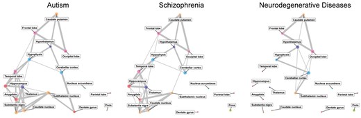
The NoN models related to ASD, SCZ and ND risk genes. The size of the node expresses the mean value of the enrichment score associated with the brain subregion (node). The smallest, middle and the largest sized nodes express below the 30-th percentile, between the 30-th and the 60-th percentiles, and above the 60-th percentile of the enrichment score across the three brain diseases, respectively. The links associated with the nodes whose enrichment scores are below the 30-th percentile are removed, as we regard them as non-related subregions. The color of the node indicates the categorization of function as determined by BTO. The thickness of the edge denotes the strength of the relation between two brain subregions. The thinnest, middle and the thickest edges express the 70-th–80-th percentiles, the 80-th–90-th percentiles and above the 90-th percentile of the coefficients across the three brain diseases, respectively

4 Discussion

In order to improve the understanding of brain-specific complex systems related to disease and to break through the limitation of network-based analyses which estimate functional single networks, we proposed a ‘Network of Networks’ approach inspired by structural equation models. In this paper, we sought to estimate the topological structure of the correlations between functional interaction networks of human brain region-specific networks associated with ASD risk genes.

To the best of our knowledge, the sparse regression for networks in GOSPEL is the first feature selection method where the features are not vectors but instead are networks. In order to construct a NoN model, GOSPEL estimates all the predictor-networks relevant to the response-network even when they have non-linear correlations. All the parameters in GOSPEL are automatically optimized by the Bayesian Optimization based on the BIC. Though there is room for improvement in that GOSPEL cannot reflect the information of the vertices (nodes), the outputted NoN model is interpretable by combining the information on the vertices and the result of community extraction, as shown in Section 3.2.1 (ii). A further limitation of GOSPEL is that all the networks must be of the same size in order to measure the correlations between networks using diffusion kernels. While overcoming this limitation is a goal for future work, we consider GOSPEL to still be useful at this stage of brain research.

We demonstrated the effectiveness of GOSPEL in simulations, and tackled the exploration of the NoN model of human brain region-specific networks related to ASD. The result was the successful production of a NoN model which shows the subregions of the brain which relate to ASD and how they functionally relate to each other. This model is consistent with previous ASD research. Although the accuracy of our model is yet untested, we hope that it will provide useful insight for ASD researchers, and that further research will prove its accuracy.

Finally, while this research was limited to the study of subregions of the brain in connection to ASD, we believe that GOSPEL will prove useful to other studies seeking to find relationships between illness and bodily organs or regions, therefore, GOSPEL may be of great use to those studying the systems of biology.

Acknowledgement

We would like to thank Makoto Yamada for helpful discussions.

Funding

This research was supported by the Japan Agency for Medical Research and Development (AMED) under the Strategic Research Program for Brain Sciences [No. JP18dm0107087], and the Japan Agency for Medical Research and Development (AMED) under Practical Research Project for Rare / Intractable Diseases [No. JP17ek0109281].

Conflict of Interest: none declared.