Network inference performance complexity: a consequence of topological, experimental and algorithmic determinants

Abstract

Motivation

Network inference algorithms aim to uncover key regulatory interactions governing cellular decision-making, disease progression and therapeutic interventions. Having an accurate blueprint of this regulation is essential for understanding and controlling cell behavior. However, the utility and impact of these approaches are limited because the ways in which various factors shape inference outcomes remain largely unknown.

Results

We identify and systematically evaluate determinants of performance—including network properties, experimental design choices and data processing—by developing new metrics that quantify confidence across algorithms in comparable terms. We conducted a multifactorial analysis that demonstrates how stimulus target, regulatory kinetics, induction and resolution dynamics, and noise differentially impact widely used algorithms in significant and previously unrecognized ways. The results show how even if high-quality data are paired with high-performing algorithms, inferred models are sometimes susceptible to giving misleading conclusions. Lastly, we validate these findings and the utility of the confidence metrics using realistic in silico gene regulatory networks. This new characterization approach provides a way to more rigorously interpret how algorithms infer regulation from biological datasets.

Availability and implementation

Code is available at http://github.com/bagherilab/networkinference/.

Supplementary information

Supplementary data are available at Bioinformatics online.

1 Introduction

The advent of genome-scale and high-throughput experiments demands network inference algorithms that accurately uncover regulation of gene expression and protein activity (Bansal et al., 2007; Bonneau, 2008; De Smet and Marchal, 2010; Marbach et al., 2010; Oates and Mukherjee, 2012). These computational tools have been invaluable for studying cell differentiation (Ocone et al., 2015), identifying genetic regulators and their targets in disease (Aibar et al., 2017; Alexopoulos et al., 2010; Gu and Xuan, 2013; Sass et al., 2015; Volinia et al., 2010) classifying diseases into subtypes (Lee et al., 2008; Wu et al., 2008), and predicting mechanisms of drug responses (Ciaccio et al., 2015; Gardner et al., 2003; Iorio et al., 2013; Korkut et al., 2015; Lecca and Re, 2016; Wildenhain, 2015).

Having a blueprint of the underlying network comprising genetic components and their regulation is essential for understanding and controlling cellular processes. Elucidating these complex blueprints directly from experimental data has proven challenging. Each algorithm offers advantages and limitations, and its reliability is shaped by biological context and experimental design. For instance, algorithms infer certain motifs with different accuracy, and so their performance depends on the presence of these motifs (Marbach et al., 2010). Such findings have helped spur efforts to benchmark algorithm performance on experimental or in silico datasets with varying properties (Chen and Mar, 2018; Hache et al., 2009; Madhamshettiwar et al., 2012; Maetschke et al., 2014; Ud-Dean and Gunawan, 2014; Zou and Feng, 2009), and some of these studies have yielded tools for further exploration of algorithm-dataset pairings (Bellot et al., 2015; Tjärnberg et al., 2017; Wang et al., 2013). Throughout, the most widely used metrics are predominantly AUROC and AUPR: the area under the receiver operator characteristic and precision-recall curves, respectively. This approach treats the inference as a binary classification, which is possible only if a gold standard network is known. However, applications with experimental data rarely have a gold standard network, making it infeasible to use AUROC or AUPR. We postulate that factors relating to network properties, experimental design and data processing affect algorithm performance, but that the type and extent of these effects remain challenging to discern, in part, because of how they typically might be assessed.

Here, we develop an in silico framework and new confidence metrics [edge score (ES) and edge rank score (ERS)], and use them to systematically evaluate the effects of kinetic parameters, network motifs, logic gates, stimulus target, stimulus temporal profile, noise, and data sampling on algorithms spanning widely used classes of statistical learning methods. The analysis distinguishes between inference accuracy and confidence, quantifies how well algorithms utilize the input data, and enables comparisons in a manner that was not previously possible. The guiding principle is that outcomes across algorithms can now be assessed in like terms through normalization to null models, which circumvents the need for a gold standard network. The results show that several factors—some within and others outside one’s direct control—exert highly significant and previously unrecognized effects, raising questions on how datasets and algorithms ought to be effectively paired. Finally, we use realistic in silico gene networks to validate our approach and apply it to tune the sensitivity and specificity of inferred models.

2 Materials and methods

Methods are detailed in Supplementary Material. Briefly, networks were formulated with logic gates for cellular mechanisms (Inoue and Meyer, 2008; Kalir et al., 2005; Mangan and Alon, 2003; Setty et al., 2003; Sudarsan et al., 2006). Target node activation was defined as a function of input nodes and affinities for the target (Ackers et al., 1982; Bintu et al., 2005; Shea and Ackers, 1985). Efficiencies for enzyme activity and gene regulation span a wide range (Bar-Even et al., 2011; Hargrove et al., 1991; Ronen et al., 2002), so varying parameter values were applied.

The panel of algorithms includes GENIE3 (Huynh-Thu et al., 2010) [which uses Random Forests (Breiman, 2001)], TIGRESS (Haury et al., 2012), BANJO (Hartemink et al., 2001; Yu et al., 2004), MIDER (Villaverde et al., 2014) and correlation (abbreviated here as CORR). We note that additional algorithms have been developed also using Random Forests (Huynh-Thu and Geurts, 2018; Huynh-Thu and Sanguinetti, 2015), regression-based methods (Bonneau et al., 2006; Ciaccio et al., 2015), dynamic Bayesian (Li et al., 2011) and information theory (Faith et al., 2007; Giorgi et al., 2014; Margolin et al., 2006; Wang et al., 2009; Zhang et al., 2013), and some approaches use multiple methods (de Matos Simoes and Emmert-Streib, 2012; Xiong and Zhou, 2012) or multiple algorithms (Madar et al., 2010; Marbach et al., 2012; Ruyssinck et al., 2014). Our focus was not to span a large number of algorithms or to determine a most effective one, but rather to evaluate determinants of performance using a concise set of established algorithms spanning different statistical methods. Therefore, and per convention, we do not include an exhaustive analysis with other algorithms, but note that the presented analysis is extensible. Additionally, we do not include algorithms intended to infer gates in large networks, but the analysis is similarly extensible, and here we indicate instances where observed trends hold across the specified gates.

Validation networks were generated using GeneNetWeaver (GNW) (Schaffter et al., 2011). Results for the five-node networks can be visualized using the online data browser at https://bagheri.northwestern.edu/browsers/networkinference/.

As described in detail in Supplementary Material, null datasets for five-node networks were generated by shuffling data across gate/motif dimensions. Null datasets for GNW networks were generated by shuffling data across nodes and stimulus conditions. To calculate ES and ERS, the necessary outcome from any method of generating the nulls is that the inferred weights (IW) and null weights (NW) are uncorrelated.

3 Results

3.1 A methodology to assess and compare algorithm performance

To identify how different factors affect inference outcomes in a controlled manner, we started by formulating in silico networks representing a range of scenarios for cellular regulation. Given the large combinatorial space, and the potential for a large network to complicate interpretation, we used a concise testbed—a strategy that has also been used in other studies (Cantone et al., 2009; Ud-Dean and Gunawan, 2014; Zou and Feng, 2009). Each network has five nodes: three (A, B, C) comprise a fan-in and the other two (D, E) are downstream of the fan-in target (C). Regulation among A, B and C is specified by a motif, and C is activated via a logic gate (Fig. 1a, Supplementary Fig. S1a–d, Tables S1 and S2). We considered 36 gate-motif combinations and four orders of magnitude of kinetic variation in gate edges. For the network inference, we chose a panel of algorithms representative of widely used statistical methods, including top performers in DREAM challenges (Haury et al., 2012; Huynh-Thu et al., 2010). The methods (and the abbreviations used here and algorithms) are Random Forests (RF, using GENIE3), least-angle regression (REG, using TIGRESS), dynamic Bayesian (DB, using BANJO), mutual information (MI, using MIDER) and correlation (CORR) (Fig. 1b).

Fig. 1.

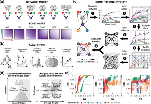
Evaluating performance of network inference. (a) Networks differ in features such as motifs and gates. Gates differentially regulate node C based on the activity of nodes A and B. Color-coding (white to purple for low to high activity) characterizes node C in the fan-in motif. (b) Panel of algorithms that use distinct statistical learning methods. (c) Networks were simulated under different conditions to produce timecourse data. Noise was added before data samples were obtained, and true data were permuted to produce null data. Regulation was inferred by each algorithm, and inferred weights (IW) and null weights (NW) were compared to determine the confidence metrics ES and ERS. (d) Left: for a true edge, the two possible outcomes from a binary classification are true positive and false negative. The IW classification threshold depends on algorithm and context. Right: four-quadrant analysis of confidence and IW suggests reasons for algorithm performance. Confidence values above 0.5 indicate that a predicted model tends to outperform null models. Ideal outcomes are in the upper-right quadrant. (e) Left and middle: analysis with IW and confidence; right: comparison of confidence metrics. Results are color-coded by algorithm. For the 36 gate-motif combinations, inference outcomes are shown that are specific to edge A →C, using: nine representative kinetic parameters (⁠$k_{\text{A}},k_{\text{B}}\in \{{10}^{-2}\hspace{0.17em}{10}^0\hspace{0.17em}{10}^2\}$⁠), stimulus to nodes A and B, no added noise, and data sampled from the full timecourse

We take a multifactorial approach to evaluate performance. Parameter values for gate edges are varied to reflect different strengths of regulation. Nodes A and/or B receive a stimulus representing the start of an experiment, such as ligand-induced pathway activation. At the halfway point, the stimulus is discontinued, representing its removal (or treatment with an inhibitor) as in the DREAM challenge (Marbach et al., 2009). Timecourse data from simulations are sampled at regular intervals, and varying levels of noise are added. Lastly, algorithms are provided for different time intervals of the data.

Importantly, as each algorithm uses a distinct statistical method and infers edge weights with different ranges and distributions, the output values cannot be directly compared. Additionally, if an algorithm correctly identifies an edge, it is not possible to determine if this outcome was discerned from information within the data or if it could have been recovered spuriously. These shortcomings motivated us to develop new, generalizable metrics to compare performance across algorithms and assess the confidence of true edges, which we arrive at by comparing IW from true data to NW from N permuted datasets (Fig. 1c). The first metric, ES, quantifies the frequency with which the true-data model outperforms a set of permuted-data models. It represents the confidence of the IW. ES for the edge from node i to node j, across N null datasets indexed by k, is given by:

$$E{S}_{ij}=\frac{1}{N}{\displaystyle \sum _{k=1}^N\left\{\begin{array}{cc}1.0,& I{W}_{ij}>N{W}_{ijk}\\ 0.5,& I{W}_{ij}=N{W}_{ijk}\\ 0.0,& I{W}_{ij}<N{W}_{ijk}\end{array}\right\}}$$

(1)

The second metric, ERS, quantifies the frequency with which an edge is more highly ranked in the true-data (predicted) model versus permuted-data models. ERS represents the confidence for if a true edge is inferred relative to other edges in a network, and is given by:

$$ER{S}_{ij}=\frac{1}{N}{\displaystyle \sum _{k=1}^N\left\{\begin{array}{cc}1.0,& \text{rank}(I{W}_{ij})>\text{rank}(N{W}_{ijk})\\ 0.5,& \text{rank}(I{W}_{ij})=\text{rank}(N{W}_{ijk})\\ 0.0,& \text{rank}(I{W}_{ij})<\text{rank}(N{W}_{ijk})\end{array}\right\}}$$

(2)

Both metrics quantify the extent to which algorithms utilize the input data. Values between (0.5, 1] indicate that the predicted model outperforms null models; 0.5 indicates equivalent performance; and [0, 0.5) indicates that null models outperform the predicted model. The use of permuted data, as opposed to randomly generated values, ensures that the null data have an overall distribution consistent with that of the true data.

To situate the new metrics in an existing framework, we consider a standard binary classification. Among the four outcomes—true positive (TP), false positive (FP), true negative (TN) and false negative (FN)—a true edge can be TP or FN (Fig. 1d, left). An algorithm that predicts true edges correctly has high recall (i.e. sensitivity), defined as TP divided by condition positive (TP + FN). However, the recall does not inform whether an algorithm truly discerns regulation based on the data or if the inference can be made by chance. To gain this insight, we use confidence to sub-categorize TP and FN (Fig. 1d, right). If IW is high and confidence > 0.5, then we deduce that the algorithm is correct for the right reasons. If IW is high but confidence < 0.5, it is correct for the wrong reasons; it guessed correctly by chance. If IW is low and confidence > 0.5, it is incorrect due to deception; it does not uncover the edge well but still outperforms the nulls, suggesting features of the data ‘deceive’ the algorithm. Lastly, if IW is low and confidence < 0.5, it is incorrect due to a difficult inference; the outcome is incorrect and has no confidence. Among the four quadrants, ideal performance is in the upper right. We note that this analysis applies to true edges. For false edges, while IW should be low, the interpretation is not defined analogously for the four quadrants.

We observed that each algorithm has characteristic trends for its IW distribution and the relationship between IW and confidence (Fig. 1e, left). For the IW values, Random Forests is low, regression is intermediate, dynamic Bayesian is binary (as expected), mutual information is clustered, and correlation is wide-ranging. Because of these differences, a low IW by one algorithm can potentially convey better edge recovery than a high IW by another, confounding direct comparisons. However, this limitation could be overcome by mapping each IW distribution onto a shared metric. To this end, we note that (i) the IW–ES relationship is monotonic for each algorithm, and (ii) for algorithms that are continuous in IW, ES surpasses 0.5 (y-axis) at a characteristic IW value (x-axis)—which in this context is 0.15 for Random Forests, 0.2 for correlation and 0.4 for regression—such that these values indicate equivalent performance compared to null models. Therefore, for a given network context, ES can be used as a common currency to directly compare IW across algorithms.

The relationship between IW and ERS is more complex than with ES, because ERS also accounts for within-model rankings. ERS can therefore capture the possibility that a low IW may convey better recovery than a high IW by the same algorithm (given a difference in motif, gate, kinetics, etc.). For example, the vertical Random Forests pattern (Fig. 1e, center) shows that one IW value can occupy different within-model rankings relative to the null expectation, and the horizontal pattern for correlation shows that different IW values can occupy similar ones. Exact trends vary across conditions (Supplemenatry Fig. S1e–g), further highlighting the distinct information captured by ERS (Fig. 1e, right). In summary, ES and ERS provide complementary information that can be applied across algorithms to augment the standard interpretation of IW.

3.2 Performance characteristics are highly variable

Given the high dimensionality of the data, we organized the simulations and inference outcomes in an online browser that allows for interactive visualization. We focus on the region where combinatorial variation was introduced and for which the results are the most informative, i.e. the fan-in edges. The kinetic landscapes for confidence show striking patterns that vary as uniform, graded, steep boundaries and speckled. The shapes of the regions for these patterns also vary as kinetically symmetric (mirror imaged across the diagonal), bounded by one or both kinetic parameters, or thin bands with linear or curved boundaries. Many landscapes have surprising combinations of features resembling phase diagrams with phase boundaries and triple points. As a representative example, we highlight a single network that produces different timecourse trajectories depending on the kinetics and stimulus (Fig. 2a), and for which algorithm performance varies as a function of kinetics, stimulus, time interval of input data and gate edge (Fig. 2b). The range of outcomes all from the same network underscores the fundamentally challenging task of network inference.

Fig. 2.

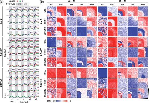
Network confidence varies across algorithms. (a) Trajectories of nodes A, B, and C, and (b) ERS for the two gate edges (A →C and B →C) for a network containing an FFFB motif and OR gate. ERS is provided as a function of stimulus condition (A only, B only or both A and B), time interval of input data (first half, second half and full timecourse), and gate kinetics (plot axes are in log space). Simulations in (a) show a subset of the kinetic landscape, and heatmaps in (b) show the full 17 × 17 landscape. Gate kinetics (a network property), stimulus target (an experimental choice), and time interval and algorithm (post-experimental choices) strongly affect inference outcomes. Additional simulation conditions and plots are in the Supplementary Material and online data browser

Despite wide variation, the results are still informative. First, much of the variation originates from decisions that in principle are within one’s control but in practice are nonobvious. For instance, confidence varies based on the employed algorithm and the time interval of input data. Additionally, stimulus choices that increase confidence in one edge are not necessarily advantageous for recovering another edge. These effects for ERS also hold for IW and ES (Supplementary Fig. S2a and b). Second, some outcomes of low confidence are due to high NW (rather than only low IW), which, in context, suggest that an algorithm would have an elevated propensity to call FPs (Supplementary Fig. S2c). For regression, NW values are relatively high, and for mutual information, NW values are low with the full timecourse dataset but high with the first and second time intervals. Lastly, each algorithm has characteristic contours in the landscapes: Random Forests, dynamic Bayesian and mutual information have defined boundaries; regression is usually highly uniform; and correlation often has several tiers. These patterns hold across networks (Supplementary Fig. S2d and e), indicating that algorithms differ in sensitivity to kinetic variation.

3.3 Differential effects of the time interval of input data and the stimulus target

Since the stimulus was applied for half of the timecourse, we considered three intervals of the data: the first half for activation, the second half for relaxation toward the initial state or continued activation, and the full timecourse. While the latter contains the most information—both in terms of data quantity and trajectory shapes—we hypothesized that the contrasting dynamics for induction and resolution of gene expression in the same dataset could potentially clarify or obscure the underlying regulation depending on the algorithm. To visualize the outcomes, kinetic landscapes are consolidated as violin plots (Fig. 3a). The results show that Random Forests performed best with the second interval and poorly with the full timecourse, and the effect was prominent. Regression often performed better with one of the two halves, and dynamic Bayesian often performed better with the full timecourse or first half. Mutual information performed best with the full timecourse and poorly with second half; full was the only one where the mean surpassed 0.5 confidence. Correlation performed best with the first half and poorly with the second, and the effect was prominent. These algorithm-specific trends hold across motifs, gates, edges and with ES (Supplementary Fig. S3a–h), demonstrating that across the networks examined here, there are certain types of dynamics from which algorithms are consistently confident or not confident. For algorithms that were most differentially affected, the time intervals for ideal performance all differed: first, second and full, for correlation, Random Forests and mutual information, respectively. Though these specific outcomes could vary across dataset contexts, the results more broadly demonstrate that providing data in greater quantity or of greater dynamical complexity does not guarantee better network models.

Fig. 3.

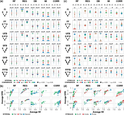
Performance depends on the sampled time interval and the stimulus target. (a) ERS distribution across the kinetic landscape for each algorithm, motif, and gate edge, with data for an OR gate and stimulus to nodes A and B. Violin plots for each landscape are color coded to reflect data sampled from the first half, second half, and full timecourse. Dashed lines indicate a confidence value of 0.5. Pairwise hypothesis testing for time intervals was performed using two-tailed Welch’s t-test, followed by multiple hypothesis correction using the Benjamini–Hochberg procedure for all tests within a given algorithm-edge group to obtain q values, as described in Materials and methods. Pairwise tests are indicated by the shapes above each subplot with statistically significant (⁠$q<0.05$⁠) outcomes filled-in. (b) Joint distribution of average IW and average ERS across the same landscape of motif-gate combinations and algorithm-edge groups. (c) ERS distribution for each algorithm, motif and gate edge, with data for an OR gate and data sampled from the full timecourse. Plots are color-coded based on node A, B, or both as the stimulus target(s). Absent violins are due to special cases that cannot be inferred (as algorithms do not interpret flat trajectories), and nonapplicable tests are denoted by a dot in place of a shape above subplots. (d) Joint distribution of average IW and average ERS. Additional simulation conditions and plots are in the Supplementary Material and online data browser

We next examined the time interval-dependent relationship between IW and ERS across more of the data (Fig. 3b). For mutual information, the best interval was primarily in the upper-right quadrant and the worst was in the lower left. For Random Forests and correlation, the best interval respectively was also in the upper right, but many low-performing cases appeared in the upper left, indicating that these algorithms were unable to infer true edges well due to misleading features of the full dataset. Distinct trends were not present for regression, indicating insensitivity to the type of dynamics in the data. Dynamic Bayesian was widely varied for the second interval and full dataset, whereas the first interval was tightly clustered. For all algorithms, the observations held for both gate edges.

Since the target node(s) of the stimulus dramatically shaped the simulations and inference outcomes, we next examined whether the choice of target node conferred specific effects (Fig. 3c). Some edges were not inferred due to flat trajectories resulting from the combination of gate, motif, and stimulus (Table S3), but in nearly all other cases, the gate edge emanating from the node that was not the target of the stimulus was inferred with greater confidence. That is, B → C was recovered with higher confidence than A → C when the stimulus targeted A, and A → C was recovered better than B → C when the stimulus targeted B. Targeting both nodes was generally disadvantageous. These trends hold across motifs, gates and algorithms, and with ES (Supplementary Fig. S3i–p). The most discernable stimulus-dependent effect on whether performance was ideal (i.e. correct for the right reasons) occurred with Random Forests and correlation (Fig. 3d). These outcomes suggest that a traditional principle—perturbing nodes to elucidate their regulation and that of downstream nodes—may come with a caveat for network inference, which is that algorithms can potentially perform worse in the topological vicinity of external interventions. As with the time interval effects, specific outcomes could vary across dataset contexts, and therefore we propose that the extent of this effect merits investigation as part of the development and benchmarking of algorithms. If it proves to be a recurring phenomenon, then an advantageous experimental strategy could be to introduce perturbations outside of the core network of interest.

3.4 Differential robustness to noise in the data

Experimental data inevitably contain noise from sources such as biological noise (Balázsi et al., 2011; Snijder and Pelkmans, 2011), cell cycle asynchrony (Buettner et al., 2015), sample preparation (Novak et al., 2002), and measurement imprecision (Stegle et al., 2015), and different noise profiles are associated with different experiments. Although methods for generating in silico data from gold standard networks often include noise (Coker et al., 2017; Mendes et al., 2003; Schaffter et al., 2011; Van den Bulcke et al., 2006), the specific ways in which this variance affects performance are poorly understood. We varied the level of noise in the data and assessed the inference outcomes (Fig. 4a), and observed that Random Forests was the least affected by noise; regression had a sharp decrease in ERS with a little noise, though additional noise had no further effect; correlation had the greatest decrease in IW; for dynamic Bayesian, the distribution of landscape-average IW values tightened; and for mutual information outcomes were varied.

Fig. 4.

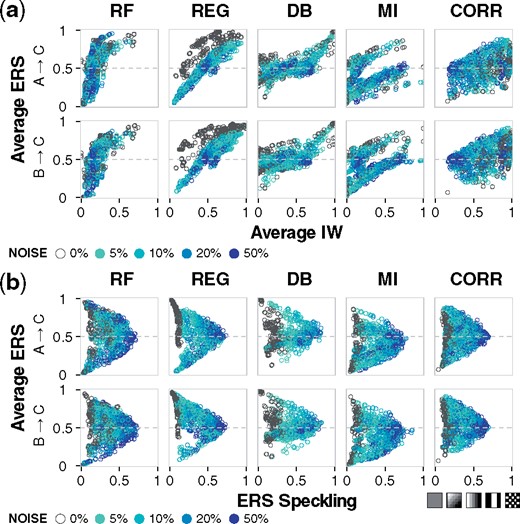
Robustness to noise in the sampled data. (a) Gaussian noise at 5, 10, 20 or 50% of the unit-scaled standard normal distribution was added to the sampled data. Joint distribution of average IW and average ERS. Each point summarizes results for a specific combination of motif, gate, stimulus target, and sampled time interval. (b) Joint distribution of ERS speckling and average ERS. With increasing levels of noise, the ERS speckling as a function of the kinetic landscape (Fig. 2b) increases and average algorithm performance converges to the null case. In the lower right, cartoon patterns depict an example trend for increased speckling. Additional simulation conditions and plots are available in the Supplementary Material and online data browser

A consistent consequence of noise was an increase in the unevenness of each algorithm’s performance across the kinetic landscape. To assess this effect, we developed a concise measure of nonuniformity that we term speckling to account for differences between all adjacent kinetic coordinates. Speckling quantifies the robustness of an algorithm to subtle variation in the data or the network from which data are collected. A uniform pattern is 0, and a checkerboard pattern is 1 (the maximum). If accuracy or confidence is highly varied between adjacent kinetic coordinates, which typically have similar dynamics, then, based on the speckling metric, we conclude that the algorithm is not robust to the variation. Without any noise, speckling was low for regression, mutual information and correlation; varied for Random Forests; and high for dynamic Bayesian (Fig. 4b). Regression had the lowest speckling and highest confidence. Notably, in all cases, as noise increases, the edge confidence approaches 0.5 (regardless of whether it is higher or lower without noise) and speckling approaches 1 (Supplementary Fig. S4). Therefore, for the cases where noise increases the average IW or confidence towards 0.5, this result can now be interpreted as an artificial inflation of confidence. We propose that a speckling analysis could allow one to identify a noise level above which performance is no longer robust, to determine whether an algorithm is reliable as a function of the estimated amount of noise in a dataset.

3.5 Resilience to kinetic and topological variation

We investigated how inference might be predictably shaped by topology and kinetics—attributes that are typically set and outside of one’s control. While none of the logic gates imparted a consistent signature to the kinetic landscapes, three motifs (FI, UFB and DFB) each did. However, despite intra-motif similarities across algorithms and edges (Supplementary Fig. S5a), consistent types of motif patterns were not discernible. This result led us to ask whether inference outcomes could be attributed more directly to the data. To this end, we note two reciprocal observations that guided the subsequent analysis: (i) many networks with the same motif and gate but different regulatory kinetics produce dissimilar data, and (ii) many networks with different motifs, gates, and/or kinetics produce similar data.

To evaluate the extent to which variation in performance is attributable to the network (topology) or the data (trajectories), we evaluated representative outcomes from the two reciprocal cases as follows: (i) if an algorithm interprets dissimilar datasets consistently, then it is robust to kinetic variation; and (ii) if it interprets similar datasets consistently, then it is robust to topological variation. For concise visualization, trajectories are condensed to their mean and standard deviation (SD), and IW and ERS outcomes are condensed to their SD. In the first case (Fig. 5a, Supplementary Fig. S5b), dynamic Bayesian and mutual information had the largest SD in confidence, followed by Random Forests and correlation. SD was generally greater for an edge across algorithms than across edges within an algorithm, indicating algorithms differ substantially in their robustness to kinetic variation. The second case showed similar outcomes for robustness to topological variation (Fig. 5b, Supplementary Fig. S5c), and this result held for ES (Supplementary Fig. S5d–e). In all, the results show that performance is affected by both factors, and algorithms differ from each other in robustness. Additionally, the second case highlights the challenge of identifiability (Oates and Mukherjee, 2012): different networks can produce similar data, and algorithms are not guaranteed to infer the correct topology even when provided low-noise time-resolved data.

Fig. 5.

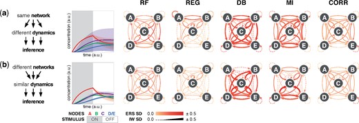
Robustness to kinetic and topological variation. (a) A network topology can produce highly distinct data depending on the kinetic parameters. In the case shown, nine networks each have a FFFB motif, an AND gate, and stimulus to node A, but differ in gate kinetics. Left: the timecourse mean trajectories (line) and standard deviation (SD; shaded region) from the nine networks. Right: SD of IW (line width) and ERS (color coded) for each edge. Dashed lines indicate zero SD for IW. (b) In the reciprocal case, nine networks differ in motifs, gates, and kinetics, but all produce highly similar data. Individual plots are in the Supplementary Material, and additional simulation conditions are available in the online data browser

3.6 Impact of modifying experimental design and algorithm implementation

Since the choice of time interval and stimulus target had significant effects, we hypothesized two strategies to produce datasets that algorithms might interpret better (Fig. 6a). The first is to modify the temporal profile of the stimulus input (‘SI’) such as with dynamic ramps or pulses. Experimentally, this level of temporal control over ligand treatment and cell signaling has been implemented using optogenetic (Toettcher et al., 2013; Zhang et al., 2014) and microfluidic (Junkin et al., 2016; Zambrano et al., 2016) techniques, though these options are not widely adopted for cell culture experiments. The second (and simpler) strategy is to provide stimulus trajectory ‘data’ for algorithms to infer regulation involving a stimulus-specific node (‘HN’ for hidden node). We hypothesized that if the influence of the stimulus could be assigned to an edge for the hidden node, then low confidence in the vicinity of the target node might be alleviated.

Fig. 6.

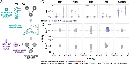
Modifications to the stimulus input and inclusion of stimulus data. (a) Depiction of the two strategies for improving algorithm performance: (i) new time-varying profiles for the stimulus input (SI), and (ii) providing stimulus information to algorithms through a new hidden node (HN). The SI panel includes ramp up, ramp down, two steps up, two steps down, two pulses, and three pulses. (b) For the HN strategy, violin plots show the IW distribution for inferred edges that are directed from the HN (shaded) or to the HN (striped), in relation to node A (purple), and nodes other than A (⁠$\neg$A, gray). Circles between the pairs of violins indicate the mean of each violin. Each violin comprises IW distributions from 20 kinetic landscapes (FF and FFFB motifs, OR and AND gates, five noise levels). (c) Individual and combined effects of the two strategies. The signed change in ERS from implementing each modification individually is indicated by the axis values. Symbols denote the SI. Combined effects are color coded as synergistic (red), antagonistic (blue), or additive (gray). (Color version of this figure is available at Bioinformatics online.)

We tested the strategies individually and in combination, first evaluating the impact the hidden node. For stimulus to node A, the expected new edge is HN → A. However, we note that in principle, performance could potentially be improved by assigning influence incorrectly via an edge from the hidden node to another node (‘$\neg$A’ for ‘not A’) and/or in the opposite direction. Since the main goal is to improve the core network model, we are more interested in the effect on the edges between original nodes, and hidden node edges could always be discarded.

The algorithm that best inferred HN →A (i.e. the true influence of the stimulus) was dynamic Bayesian (Fig. 6b). GENIE3, regression and mutual information almost never detected it, and while correlation usually did, the $\neg$A edges had higher IW. Next, we examined the consequences of the hidden node with the SI panel, and whether the strategies’ combined effects were synergistic, antagonistic or neither (strictly additive) (Fig. 6c). The hidden node had no effect on correlation (as expected), modest effects on Random Forests and regression, and larger, often positive effects on dynamic Bayesian and mutual information. Changing the SI had modest effects on correlation, Random Forests and regression; large and varied effects on dynamic Bayesian; and generally improved effects on mutual information. While the effects of certain SI were wide ranging, the ramp up profile was the most likely to improve A →C ERS (Supplementary Fig. S6). Therefore, for certain algorithms, there may be steps that can be taken, in experimental design and in how data are provided to algorithms, to improve inferred models. However, in general it appears that algorithms are insensitive to such strategies.

3.7 Validation of the metrics using 50-node networks

To investigate the application of the confidence metrics, we extracted and analyzed 50-node networks from the yeast transcriptional regulatory network using GNW. For each network, nodes were individually stimulated, and timecourse data were collected and provided to algorithms. Since the option to shuffle data across motif-gate combinations was unavailable in this context, null trajectories for the null models were instead generated by shuffling across nodes and stimulus conditions, in a manner that could also be performed with experimental data (Materials and methods). We observed similar overall trends for the metrics compared to the five-node networks (Fig. 7a, Supplementary Fig. S7a), and that the monotonic IW–ES relationship was maintained (Fig. 7, left, Supplementary Fig. S7b). Additionally, we found that for NW and IW to be uncorrelated (Fig. 7a, right; a necessary condition for calculating confidence metrics), the null trajectories needed sufficient variation. Therefore, generation of the nulls requires empirical assessment to ensure their suitability. The large amount of shuffling of the GNW data ensured suitability of the nulls, and as a side effect the NW values are lower and the IW–ES relationship is steeper than for the five-node networks. Importantly, these differences do not prevent the analysis of interest, as comparisons between algorithms are intended only within each network context.

Fig. 7.

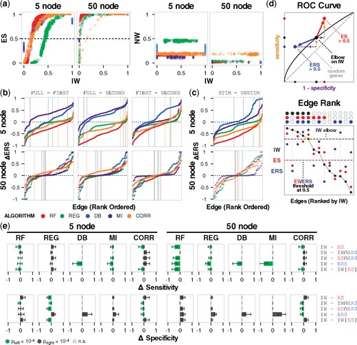
Validation using GeneNetWeaver networks. (a) IW–ES and IW–NW relationships for the original 5-node and validation 50-node networks, color-coded by algorithm. (b) Rank-ordered differences in ERS of two-parent fan-in edges between each pair of time intervals used as input data. Vertical lines indicate the x-coordinate where each trace changes sign. (c) Rank-ordered differences in ERS of two-parent fan-in edges when the parent node does or does not receive the stimulus. (d) Diagram depicting the principle of using different metrics to threshold edges in an inferred model. Upper: modulating the sensitivity-specificity trade-off without the constraint of remaining on the ROC curve. The larger arrows illustrate general trends using ES > 0.5 and IW$\cap$ERS > 0.5, but there are also other possible directions. Movement for the former depends on the initial location of comparison on the ROC curve, and movement for the latter is in a direction of lower sensitivity and higher specificity. Lower: in standard thresholding, edges are rank-ordered (x-axis) by value (y-axis) of IW (black) and only edges above the elbow are retained. Alternatively, ES (red) or ERS (blue) can be used, in combination with each other or IW, to retain high-confidence edges. Above the plot, filled-in circles indicate edges selected based on IW > elbow threshold, ES > 0.5, and ERS > 0.5. (e) Average difference in sensitivity and specificity using IW versus other approaches (rows). Error bars indicate standard deviation. Statistical significance from a one-tailed Wilcoxon signed-rank test is color coded. For example, if thresholding by ES > 0.5 gives significantly greater specificity than elbow-thresholding IW, this outcome is depicted by a green bar to the left of the zero coordinate. (Color version of this figure is available at Bioinformatics online.)

We next revisited some of the phenomena from the five-node analysis. As the time interval of input data and the stimulus both affected confidence (Figure 3), we visualized the rank-ordered effects on ERS for two-parent fan-in edges. Although the mean effect magnitudes were lower for GNW, a substantial proportion of edges were still affected (Fig. 7b and c, Supplementary Fig. S7c), reinforcing that these experimental design choices have substantial and potentially unpredictable consequences.

Finally, we asked whether ES and ERS could be applied to inferred models post hoc by informing which edges to keep versus discard. The standard approach for enforcing edge sparsity is to set a threshold for IW (e.g. based on an elbow, which refers to a sharp drop-off in a plot of rank-ordered IW values) and retain edges that pass the threshold, although there is no standard way to identify the location of the threshold. If the threshold permits too many edges, a model will tend to recover regulation with high sensitivity but low specificity, and if it is too stringent the result will be high specificity but low sensitivity. If the gold standard is known, this trade-off is described by the ROC curve, which represents possible models starting at the lower-left and extending to the upper-right as the threshold is relaxed (Fig. 7d, upper). An ideal model is in the upper-left corner, where specificity and sensitivity are both 1. For experimental applications, the gold standard, ROC curve and location in ROC space are unknown. However, we reasoned that it would still be useful to be able to make controlled movements, such as when a given application could benefit from erring on the side of greater sensitivity or specificity. Therefore, we examined whether ES or ERS could be used to traverse upward (higher sensitivity) or leftward (higher specificity) in a principled manner, without knowing the gold standard, and without the constraint of the ROC curve. We note that the ROC curve in Figure 7d is shown as a visual depiction for the subsequent analysis, and a PR curve would illustrate the same concept.

As a base case against which to compare each new post hoc procedure, the IW threshold for each model in the 5-node and 50-node sets was determined using the elbow rule (Materials and Methods), and sensitivity and specificity were calculated based on the true network represented by the provided dataset. Since the rank order of edges differs between metrics (Supplementary Fig. S7d and e), we hypothesized that post hoc decisions based on ES, ERS or combinations of metrics might produce networks with different properties than the base case (Fig. 7d, lower). We evaluated three new methods relative to the base case (elbow on IW). In the visualization, deviation from zero denotes an increase or decrease (Fig. 7e). Outcomes were similar between the 5-node and 50-node networks, indicating that the observed trends hold for larger networks. For Method #1, networks with edges based on the criterion of ES > 0.5 had increased sensitivity (with an exception for TIGRESS in the five-node case), indicating that the standard IW elbow tended to exclude some high-confidence edges. Importantly, ES > 0.5 represents a single point as opposed to a curve in sensitivity-specificity space, and it can be distinct from but is generally in the vicinity of the ROC curve. The 0.5 criterion is derived from the definition of ES and is less subjective than, for example, identifying an elbow for IW. Method #2 used the intersection of edges satisfying elbow-thresholded IW and ERS > 0.5, creating a curve of sparser networks with lower sensitivity and higher specificity. Method #3 used the intersection of ES > 0.5 and ERS > 0.5, and the outcomes are a point as with Method #1.

The fourth and fifth rows are controls. The fourth (ERS > 0.5) shows that: (i) ERS provides some information that is distinct from ES and (ii) the increased specificity in Methods #2 and #3 is due to the use of ERS in combination with other metrics. In the fifth row, IW was thresholded at the same number of edges obtained with Method #1. The similarity of the first and fifth rows are due to a comparable rank ordering of edges by IW and ES, as expected from their monotonic relationship. We then extended this control to the other cases and observed that there were statistically significant differences in sensitivity and specificity (Supplementary Fig. S7f). While outcomes could generally be ascribed to tuning the specificity-sensitivity trade-off, there were cases with different rank ordering between IW, ES and ERS, and thus there was movement off of the ROC curve as anticipated. In summary, ES and ERS can be used to evaluate performance of inference algorithms in like terms, and they can also be applied to tune inferred models post hoc on the basis of how well algorithms recover regulatory interactions from true data relative to null data without relying on a gold standard.

4 Discussion

This study develops a way to evaluate the confidence and robustness of inference outcomes, which is enabled through comparisons to null models. While the analysis utilizes in silico data with many timepoints, it can also be applied to experimental datasets with fewer timepoints, and in principle it is extensible to any algorithm. Overall, we find that performance is significantly shaped by previously unrecognized factors, some within and others outside of one’s control. To promote exploration of the multidimensional analysis, we produced an interactive online browser. The results show how (i) kinetic parameters affect outcomes in complex ways; performance can be affected (ii) by the type of dynamics portrayed by the data and (iii) in the topological vicinity of a stimulus; (iv) algorithms differ in robustness to deviations in data arising from kinetic variation or noise; (v) topological and kinetic variation have similar effect magnitudes, which vary by algorithm; and (vi) there are ways to improve performance under some conditions, but it remains to be seen whether there are more corrective steps. Given the impact of these factors, we suggest they could be considered more broadly in the benchmarking of algorithms.

While there has been progress in creating, comparing, and refining algorithms, fundamental questions remain on how algorithms ought to be used and how models ought to be interpreted. Our results indicate that, counterintuitively, the pairing of high-quality data with high-performing algorithms can still produce inaccurate models. With the new metrics, a four-quadrant analysis provides an interpretation for why some dataset-algorithm combinations do well and others do not. In cases where the gold standard is known, established metrics such as AUROC and AUPR can be used to quantify outcomes. If the gold standard is unknown, as for applications with experimental data, ES and ERS provide standard approaches to select edges in a network model. For the method with ES > 0.5, this defined threshold circumvents the need to identify an IW elbow (a somewhat arbitrary threshold) and may produce high-confidence models that balance sensitivity and specificity. Using ERS in combination with IW filters out highly ranked edges that are also highly ranked in null models, potentially removing FPs.

The no free lunch theorems for optimization (Wolpert and Macready, 1997) state that one should expect identical average algorithm performance in the limit of all possible problems, but that some algorithms will outperform others if better aligned with the subset of problems at hand. In this light, network inference applications would benefit especially from a greater understanding of the types of data that algorithms interpret well and the circumstances under which experiments can produce data that align with these criteria. Achieving this goal will require experimental design (e.g., stimulus target/profile and number/spacing of measurements) that is based, in part, on how well the experiments position algorithms to extract information. Reciprocally, this goal will also require more study on which algorithms effectively utilize data portraying characteristic features of gene regulation and cell signaling. Ultimately, further characterization of the factors that benefit and hinder algorithms, and investigation on how data and algorithms should be paired, will enable more accurate models and their effective applications.

Funding

This work was supported in part by a Northwestern University Biotechnology Training Program cluster award to J.J.M., National Science Foundation GRFP award to J.S.Y., National Science Foundation CAREER award to N.B. (CBET-1653315), and the Northwestern University McCormick School of Engineering. We acknowledge the computational resources and staff contributions provided for the Quest high-performance computing facility at Northwestern University, which is jointly supported by the Office of the Provost, the Office for Research, and Northwestern University Information Technology.

Conflict of Interest: none declared.

Author notes

The authors wish it to be known that, in their opinion, Joseph J. Muldoon and Jessica S. Yu authors should be regarded as Joint First authors.