Predicting runtimes of bioinformatics tools based on historical data: five years of Galaxy usage

Abstract

Motivation

One of the many technical challenges that arises when scheduling bioinformatics analyses at scale is determining the appropriate amount of memory and processing resources. Both over- and under-allocation leads to an inefficient use of computational infrastructure. Over allocation locks resources that could otherwise be used for other analyses. Under-allocation causes job failure and requires analyses to be repeated with a larger memory or runtime allowance. We address this challenge by using a historical dataset of bioinformatics analyses run on the Galaxy platform to demonstrate the feasibility of an online service for resource requirement estimation.

Results

Here we introduced the Galaxy job run dataset and tested popular machine learning models on the task of resource usage prediction. We include three popular forest models: the extra trees regressor, the gradient boosting regressor and the random forest regressor, and find that random forests perform best in the runtime prediction task. We also present two methods of choosing walltimes for previously unseen jobs. Quantile regression forests are more accurate in their predictions, and grant the ability to improve performance by changing the confidence of the estimates. However, the sizes of the confidence intervals are variable and cannot be absolutely constrained. Random forest classifiers address this problem by providing control over the size of the prediction intervals with an accuracy that is comparable to that of the regressor. We show that estimating the memory requirements of a job is possible using the same methods, which as far as we know, has not been done before. Such estimation can be highly beneficial for accurate resource allocation.

Availability and implementation

Source code available at https://github.com/atyryshkina/algorithm-performance-analysis, implemented in Python.

Supplementary information

Supplementary data are available at Bioinformatics online.

1 Introduction

1.1 Purpose

Galaxy (at http://galaxyproject.org) is a platform that allows researchers to analyze large biological datasets and run popular bioinformatics analyses on high performance computing infrastructure (Afgan et al., 2016; Blankenberg et al., 2010; Goecks et al., 2010). In particular Galaxy’s main North American site at http://usegalaxy.org leverages high performance computing provided by the Extreme Science and Engineering Discovery Environment. A challenge faced by administrators of this (and many other) Galaxy instances is coordinating the high throughput of analysis requests and efficiently completing them.

Currently, the administrators of Galaxy main site use tool-specific heuristics to estimate the time and space requirements of a job. Most jobs have a flat allocation of 32 Gb of RAM and a walltime of 72 h. This varies depending on the known behavior of the tool in question. In addition, there is a computer cluster dedicated for large jobs (e.g. genome and transcriptome assembly) that provides unlimited amount of runtime and 128 Gb of memory. These heuristics are undoubtedly naive. To find a more intelligent way of assessing resource allocation we sought to leverage the historical dataset of job runs that have been collected over the past 5 years.

In the case of space and time allocation, the Galaxy main administrators choose to overestimate the amount required by a job to prevent failures due to memory overflow or timeout. An accurate estimate of the amount of memory and time required by a job will allow administrators to more efficiently allocate resources and increase the volume of jobs processed by the server.

If resource usage estimation is possible cross-platform, an online estimation service will be of use to administrators of other Galaxy instances and to independent users of bioinformatics software. As of yet, cross-platform experiments have not been performed, but the results presented in this paper are promising for a single platform service.

1.2 Previous work

The prediction of runtimes of complex algorithms using machine learning approaches has been done before (Duan et al., 2009; Gupta et al., 2008; Hutter et al., 2006; Matsunaga and Fortes, 2010; Nadeem and Fahringer, 2009; Phinjaroenphan et al., 2005; Sonmez et al., 2009). Typically, these prediction models have been built on datasets of jobs run on identical hardware. The popularity of cloud computing has also stimulated activity in the problem of resource usage prediction (Bankole and Ajila, 2013; Gong et al., 2010; Islam et al., 2012). The methods developed for cloud computing, however, scale virtual machines with no knowledge of the programs or algorithms that are being run. The predictions are based on traffic and usage patterns at discrete time steps. Since we are not interested in predicting resource usage based on time usage patterns, we forego these methods.

The most comprehensive survey of runtime prediction models was done by Hutter et al. (2014). These authors compared 11 regressors including ridge regression, neural networks, stochastic gradient descent and random forests. They found that the random forest outperforms the other regressors in nearly all runtime prediction assessments and is able to handle high dimensional data without the need of feature selection. Based on these results we have chosen random forest approach as the general framework for solving our problem.

In our paper, we compare the performance of the classical random forest against two variations: extra random trees and gradient boosting. We consider the use of quantile regression and classification for walltime and maximum memory usage estimation. Finally, we discuss the plausibility of an API that provides resource use estimation for Galaxy jobs.

2 Results and discussion

2.1 Random forests

We will briefly describe random forests (Breiman, 2001) as they are fundamental to the methodology used in this paper. A random forest is a collection of decision trees. A decision tree is a flowchart that accepts an object with known attributes as an input in order to guess an unknown attribute of the object. The object begins at the root node of the tree, and the unknown attribute guesses are stored in the leaf nodes. At each node of the tree (except for the leaf nodes) a test is performed on an attribute of the object in question, and the result of that test determines to which node the object traverses. Once the object reaches a leaf node, the value stored in the leaf is the decision tree’s prediction of the object’s unknown attribute. An example of a simple decision tree can be seen in Figure 1, in which the input object is a job and the unknown attribute is the runtime of the job. At each node an attribute of the job is tested. For instance, the root node tests the input data size is greater than or lesser than a certain amount.

Fig. 1.

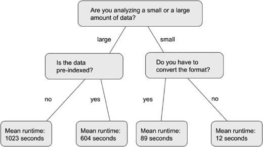
Control flow of a short decision tree. The root node is at the top, and the leaf nodes are at the bottom

The decision tree’s control flow is determined by training on a set of objects. Training begins with all of the objects at the root node. It then considers at a subset of attributes and a subset of object instances of the dataset, and chooses to split the data in the way that minimizes variability of the attribute of interest in the subsequent two nodes. This split corresponds with the attribute test used later to make decisions. In this way, the tree sorts objects by similarity of the attributes. Once the tree is trained, it can then be used to predict the unknown attributes of previously unseen objects.

A random forest is a collection of decision trees, each of which are trained with a unique random seed. The random seed determines on which sub-sample of the data each decision tree is trained and which sub-sample of data each node of each tree uses when making decisions. By implementing these constraints, the random forest protects itself from overfitting—a problem to which decision trees are susceptible.

A random forest can be used as either a classifier or a regressor. As a classifier, the trees vote on the correct class attribute, and the class that is voted for the most is the forest’s prediction. As a regressor, a weighted average of the tree’s predictions is taken to be the forest’s prediction.

There are other variations to the random forest. We use a few variations, such as extra trees and gradient boosting, in this work and describe them further in the Section 4.

2.2 Data collection

The main public server of the Galaxy has been collecting extensive job run data on all analyses since 2013 (memory data collection has begun in early 2018). These data represent the largest, most comprehensive dataset available to date on the runtime dynamics for some of the most popular biological data analysis software (a summary for tool popularity and the relationship between the number of errors and the number of jobs are shown in Supplementary Figs S1 and S2, respectively). This large collection of job runs with attributes can be leveraged to determine more efficient ways for allocation of server resources.

The job run attributes collected by the Galaxy can be seen in Table 1. Generic information about each job are collected, such as tool used, job creation time, and basic hardware attributes. In addition to this, job specific attributes are collected. For the data used to generate the runtime prediction models, we supply Supplementary Material 1 which was generated by the steps outlined in the Sections 4.5 and 4.6. For the data used to generate the memory prediction models, we supply Supplementary Material 2 which contains the attributes used to train the memory usage prediction models for the four tools that were tested.

Table 1.

Job attributes tracked by the Galaxy main server

Attribute group	Attributes
Job Info	Id
	tool_id
	tool_version
	state
	create_time
Numeric metrics	processor_count
	memtotal
	swaptotal
	runtime_seconds
	galaxy_slots
	start_epoch
	end_epoch
	galaxy_memory_mb
	memory.oom_control.under_oom
	memory.oom_control.oom_kill_disable
	cpuacct.usage
	memory.max_usage_in_bytes
	memory.memsw.max_usage_in_bytes
	memory.failcnt
	memory.memsw.limit_in_bytes
	memory.limit_in_bytes
	memory.soft_limit_in_bytes
User selected parameters	Tool specific
Datasets	ob_id
	dataset_id
	extension
	file_size
	param_name
	type (input or output)

2.3 Model comparison

In this work, we were first interested in comparing models in the task of runtime prediction, including two regression models that had not been tested by Hutter et al. (2014): extremely randomized trees and gradient boosting. These two forest methods have comparable performance to random forests in many tasks, which is why we were interested in measuring their performances.

As seen in Figure 2, the random forest, the extra trees regressor and the gradient boosting regressor have comparable performances, but the random forest performs slightly better. We also are able to verify that the random forest outperforms other regressors that were tested by Hutter et al. (2014) Those results are not presented here. The performance of all of the regression models in the task of runtime prediction can be seen in Supplementary Table S1.

Fig. 2.

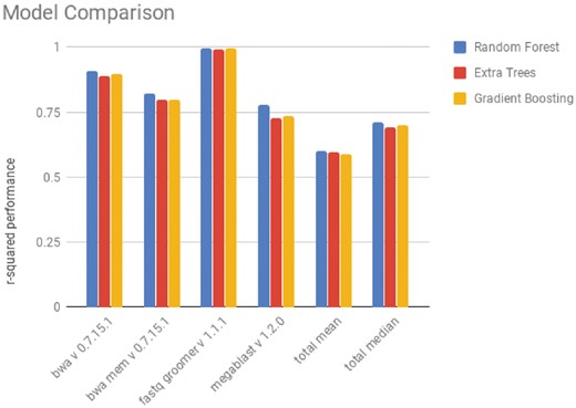
Performance of regression models on the prediction of runtime of jobs. The performance metric used is the coefficient of determination (r 2). The value displayed is the mean value of a 3-fold validation. The total mean and median were taken as the performance of the tool over every tool with more than 100 recorded runs

2.4 Estimating a range of runtimes

Estimating a range of runtimes the random forest gave us the best results for estimating the runtime of a job. It is also be of interest to calculate a confidence interval for the runtime of a job, so that, when using the model to choose walltimes, we lower the risk of ending jobs prematurely. We used a standard deviation random forest as described in the Section 4.

As seen in Figure 3a, the performance of the standard deviation random forest increases with the size of the confidence interval. However, as the accuracy increases, the precision decreases. In addition, as seen in Figure 3b, the precision of the predictions varies between tools. This indicates that some tools have more consistent runtime behavior given a set of user-selected parameters. The cause of this may be a combination of several factors: the amount of historical data to train on, the variability in user-selected parameters and the amount and effect of bifurcations in the algorithm.

Fig. 3.

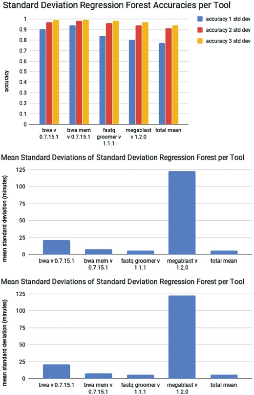
(top) Performance of a random forest modified to calculate standard deviations. (middle) Average size of on standard deviation predicted the random forest on the testing set over 3-fold cross validation. (bottom) Distribution of standard deviations output by the standard deviation forest for predictions of Megablast runtimes

The confidence intervals produced also vary between job instances, as seen in Figure 3c. The largest drawback of the quantile regression forest is this lack of control over the time ranges that are produced. The predicted time range sizes are volatile, and can vary from seconds to hours. The sizes of the confidence intervals can be scaled with the confidence factor, but they cannot be absolutely constrained. Large time ranges perhaps may be useful to administrators creating walltimes, but they are not be useful approximating the length of time needed for an analysis to complete within a reasonable time window. To counter the volatility of the sizes of the confidence interval made by the standard deviation random forest, we tested the performance of a classifier. With a classifier, we can specify the runtime intervals to be used. We choose the runtime intervals as described in the Section 4.

The performance of the standard deviation regression forest and the random forest classifier for all of the tools can found in Supplementary Tables S2 and S3, respectively. A comparison of the performance of the two methods on a select number of tools can be seen in Figure 4a. The performance of the classifier is comparable to the performance of the regression forest when a confidence of 1 SD is used. The sizes of the runtime intervals are similarly comparable to the sizes of confidence intervals produced by the regression forest when 1 SD is used (Fig. 4b). However, when the size of the standard deviation is increased, the regression forest begins to outperform the classifier. Because of their close level of performance, the choice of which model to use depends the goal of the project. If the importance of constraining the maximum prediction window size is greater than the importance of accuracy, then a classifier may be more suitable. Conversely, a regression forest with a static runtime interval may also suit those purposes with similar accuracy. For our project, we favor the accuracy provided by the standard deviation regression forest.

Table 2.

Performance of random forest on predicting the memory requirements of tools

Tool	Number of jobs in dataset	r2 score (mean)	Accuracy: 1SD	Accuracy: 2SD	Accuracy: 3SD
bowtie2	3985	0.95	0.77	0.95	0.99
hisat2	2811	0.96	0.70	0.92	0.96
bwa mem	2199	0.78	0.71	0.93	0.97
stringtie	1399	0.90	0.68	0.89	0.94

Fig. 4.

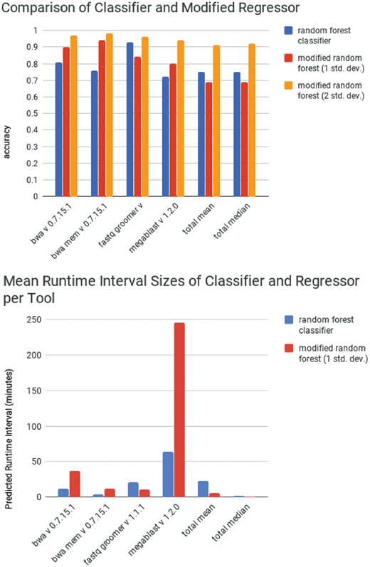
(top) Performance of a random forest classifier compared to the performance of a random forest modified to calculate standard deviations. (bottom) The average size of classified runtime range predicted by the random forest classifier compared to one runtime range predicted the random forest on the testing set over 3-fold cross validation

2.5 Memory requirement prediction

Galaxy Main began collecting memory use data in early 2018. Because of this, the dataset of memory usage of jobs is not as large as that for runtimes. Consequently, we will focus on a subset of the most popular jobs for our predictive models. We use a modified regression forest which, as far as we know, has not been tested on space resource requirements estimation before.

As can be seen in Table 2, the performance of the regression forest in this task is similar to its performance in the runtime prediction, achieving about 0.9% accuracy with the use of a confidence interval of 2 SD. It is important to note here that the dataset of memory usage of jobs was collected over the course of one month. This may have led to a less representative sample of the possible behavior of the tools, and an inflated accuracy for these tests.

Shown in Figure 5 are sample predictions of the standard deviation regression forest in the task of memory requirement prediction. The figure was produced by training the models on a random sample of 80% of the recorded jobs of a tool and testing the models on the remaining 20% of jobs. The confidence interval of 2 SD was used, as it gave reasonable results with performance hovering around 0.9 for most of the tools. The results are an encouraging step to the goal of an online memory resource estimation service.

Fig. 5.

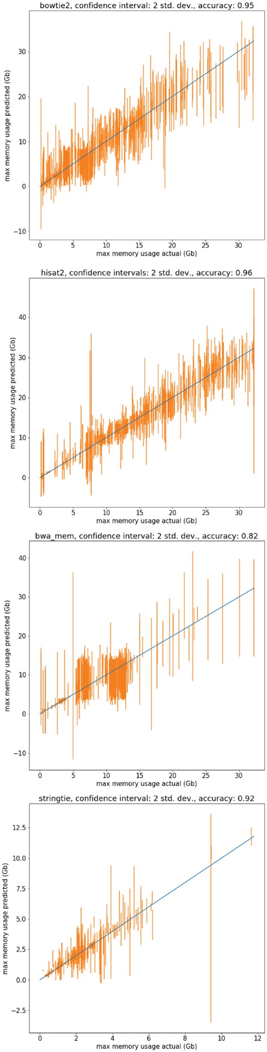
Actual maximum memory usage versus predicted memory usage of the modified random forest with confidence intervals of 2 SD. The models were trained on a random sample of a training set consisting of 0.8 jobs of the dataset, and the predictions shown are on the remaining 0.2 jobs of the dataset. The tools shown are (top) bowtie2, (middle) hisat2, (bottom) bwa mem and (respectively) stringtie

2.6 Walltime and memory requirement estimations via an API

It is beneficial for Galaxy server administrators to know the resource requirements of a job before it is run. Allocating the appropriate computational resources, without using more than necessary, would lead to shorter queue times and more efficient use of resources.

First, we will discuss the possibility of an online runtime estimation service. One item that we had glossed over earlier is that the runtime of a job is hardware specific. It depends on the CPU clock, CPU cache, memory speed and disk read/write speed. Because of the high variability in server hardware configurations, it is unclear whether a runtime prediction service would be accurate across different servers, as these tests still need to be completed. An alternative solution to an online service is an addition of a package to the Galaxy code base that would allow Galaxy administrators to train unique models on their own job run histories. The drawback is that Galaxy instances that have a smaller user basis may be lacking in the training data to build such models. It is of interest, therefore, to complete these tests to determine to feasibility of a cross-server runtime estimation model.

On the other hand, maximum memory usage of a job is mostly hardware independent. This is of benefit, since we can then train one random forest (per tool) on jobs across all the Galaxy servers to create a more robust model. The one concern with this proposal is that some Galaxy servers are tailored for specific analyses. One Galaxy instance may process more bacterial genome alignments, whereas another Galaxy instance processes more plant genomes. The differences in the omics in the different groups of organisms may cause difficulty in creating a universal memory estimation service, and begs for more cross-Galaxy instance tests. Still, a generic online estimation service is certainly feasible for generic Galaxy instances such as Galaxy Main and Galaxy Europe.

2.7 Application to real world job scheduling

Jobs on Galaxy Main (http://usegalaxy.org) are managed a distributed resource manager (DRM), Slurm (https://slurm.schedmd.com/). DRM software provides cluster scheduling and execution functionality. When jobs are submitted for execution, the submitter can specify the job’s maximum allowable run time (‘walltime’), as well as the required number of number of CPU cores and amount of memory. Once a job is queued, the DRM decides when jobs should be allocated nodes, and which nodes to allocate, based on multiple factors, including the requested cores/memory and walltime.

In a simple configuration where all jobs are homogeneous with respect to requested walltime and cores/memory, the DRM schedules jobs using a simple first-in first-out algorithm. Currently on Galaxy Main, all jobs for tools that are able to run in parallel on multiple cores are submitted with a walltime of 36 h, and are allocated six CPU cores and 30 GB of memory. Slurm will assign these to nodes in the order in which they are received. If a job is enqueued and there are not enough free cores or memory to allocate, that job, and all jobs submitted after it, will remain queued until resources become available.

More complex scheduling algorithms are possible when jobs vary in their requested limits and resources, which can yield higher throughput, lower wait times and better utilization of compute resources. This is done primarily through an algorithm commonly referred to as backfill scheduling. Consider a scenario in which the cluster consists (for the sake of example) of only a single 12 core node with 64 GB of memory. On this node, two jobs are running: Job A, allocated 6 cores and a 12 h walltime, has been running for 4 h, and Job B, allocated 4 cores and a 8 h walltime, has been running for 2 h. With a total of 10 cores in use, this leaves 2 cores on the node standing idle. Also for the sake of example, assume that jobs run for their entire walltime, and no less. Next, two new jobs are enqueued: first, job C requiring 6 cores and having a walltime of 12 h, and second, job D requiring 2 cores and having a walltime of 30 min. Using first-in first-out scheduling, despite there being adequate cores free, job D will not be allocated resources until: (i) Job B completes, (ii) Job C is scheduled and (iii) Job A completes. This is 8 h from the time of submission of job D.

Using backfill scheduling, however, the DRM sees that no job is expected to finish within the next 6 h, and therefore, it can schedule and complete job D immediately. Job C will run at the same time as it would have otherwise. In a real world scenario where jobs can finish before their runtime, the worst case scenario is that job C starts a short time after it would have had job D not been backfilled, so the negative impact of backfilling is quite low. Thus, having accurate runtime predictions allow for significant improvements in job throughput and a reduction of user wait times.

3 Future work

In addition to performing cross-server tests to determine the transferability of the resource prediction models, we are also interested in studying effect of parallel processors on runtime. Currently, every job on Galaxy main that can be run on parallel processors is allotted six processor cores. Because of this, we do not have the historical data to investigate the effect of core count on runtime. Adding random fluctuations to the allotment of cores will be the place to start. Once this is done, analyses may be completed to determine if there is an optimal number of cores a tool, or job, should be allocated.

4 Materials and methods

4.1 Caveats of data collection

There are several caveats associated with the historical dataset of jobs runs. Galaxy Main has three server clusters to which it sends jobs. The clusters have different hardware specifications and underlying configurations. Because the jobs are run on a remote site, the Galaxy Main instance does not know which hardware is assigned to which job. In addition, The CPUs of the nodes are shared with other jobs running concurrently, so the performance of jobs is also affected by the server load at the time of execution. These attributes are not in the dataset because of the difficulty of tracking them.

4.2 Undetected errors

A hurdle the job run dataset presents is that it contains undetected errors—errors that occurred but were not recorded. One type of undetected error is the input file error, in which jobs are recorded to have completed ‘successfully’ without the requisite input data. For instance, there are 49 jobs of the tool bwamem Galaxy version 0.7.15.1 that completed successfully without the requisite input. This comprises.25% of ‘successful’ jobs recorded for this tool. Whether these errors are caused by bugs in the tool code, malfunctions in the server, mistakes in record keeping or a combination of these, the presence of these of errors casts uncertainty to the correctness of other anomalous instances in the dataset. If there are many jobs similarly mislabeled as ‘successfully completed’ that are not as easily identified as are input file errors, it will bias the predictions and the performance metrics, which are computed on the same, possibly flawed, dataset.

In order to deal with the questionable job runs, we tested two methods of removing undetected errors: the exclusion of extreme values and the exclusion of anomalies detected by an isolation forest. We tested the methods in two ways: visually by plots and by the effect of removal of the outliers on the performance of the models.

Visually, we expect certain correlations to appear between input data and runtime—as the size of input data increases, so should the runtime. Both methods failed at removing the anomalous instances that were seen in such plots. As for model performance, the performance of the prediction models did not change significantly when using a dataset trimmed by either method. For these reasons, we did not implement either method to remove anomalous job instance in this project and opted for using the full dataset.

4.3 Variations of the random forest

We use a few variation of the random forest. Here, we describe them in the order they appear in the text.

Extremely randomized trees (Geurts et al., 2006) and gradient boosting (Friedman, 2001) are two forest methods that have comparable performance to classical random forests on many tasks. Extremely randomized trees are a forest model with a modification in how the trees are trained. The extremely randomized trees will choose the best split over a sub-sample of random splits, where ease a random forest will choose the best split over a sub-sample of the dataset that it is using. The gradient boosting model uses shallower trees than the random forest, and the trees are trained sequentially. The construction of one tree is built by taking the negative gradient of the cost function of the previous trees.

Next, we describe the isolation forest (Ting et al., 2008), which is a forest model that is used for anomaly detection. In an isolation forest, the data are split based on a random selection of an attribute and split. The shorter the path to isolate a data instance, the more likely that it is an anomaly. The data instances with the shortest average isolation paths are considered to be the outliers.

Finally, we discuss the quantile and standard deviation regression forests. A quantile regression forest (Meinshausen, 2006) and a standard deviation forest (Hutter et al., 2014) can each be used to calculate confidence prediction intervals. A quantile regression forest can be trained the same way as a random forest, except that at the leaves of its trees, the quantile regression forest not only stores the means of the variable to predict, but all of the values found in the training set. By doing this, it is able to calculate a confidence interval for the runtime of a job based on the quantile chosen.

However, storing the entire dataset in the leaves of every tree can use a large amount of memory. For this reason, we used a standard deviation regression forest instead. A standard deviation regression forest only stores the means and the standard deviations in its leaves. Doing so reduces the precision of the confidence interval, but saves space.

In this work, we use the random forest implementation provided by the scikit-learn library (Pedregosa et al., 2011). We also use scikit-learn library for the extra trees regressor, the gradient boosting regressor and the isolation forest. We use the implementation provided in the expanded scikit-garden library for the standard deviation random forest.

4.4 Model parameters

The random forest, extra trees and isolation forest models used in this project each exhibit 100 trees and a maximum depth of 12. The gradient boosting models used in this project exhibit 100 trees and a maximum depth of 3.

For the random forest classifier, we chose buckets in the following manner.

• We ordered the jobs by length of runtime.

• Then, we made (0, median) our first bucket.

• We recursively took the median of the remaining runtimes until the number of remaining bucket held <100 instances.

For example, for bwamem the buckets we found (in seconds) were (0, 155.0, 592.5, 1616.0, 3975.0, 7024.5, 10523.0, 60409.0). As the buckets become larger the number of jobs in the bucket decreases. For bwamem, the last bucket holds only 0.78% of the jobs. Dividing it further would make it so the next bucket created has <100 jobs, which we chose as the threshold.

4.5 Feature selection

Galaxy records all parameters passed through the command line. This presents in the dataset as a mixed bag of relevant and irrelevant attributes as seen in Table 1.

For a few, popular tools, we manually select which parameters to use. However, since we have many tools, with incongruous naming schemes and unique parameters, we cannot do this for each tool.

Instead, we created a heuristic to eliminate common irrelevant features. The simple heuristic attempts to remove any labels or identification numbers that are present. Although it does not search for redundant parameters, it can be altered to do so.

The parameters are screened in the following way:

1. Remove likely irrelevant parameters such as:

   • workflow_invocation_uuid

   • chromInfo

   • parameters whose name begins with

     • job_resource

     • rg (i.e. read groups)

     • reference_source (this is often redundant to dbkey)

   • parameters whose names end with

     • id

     • indices

     • identifier

2. Remove any non-numerical parameter whose number of unique values exceeds a threshold

3. Remove parameters whose number of undeclared instances exceed a threshold

4. Remove parameters that are list or dict representations of objects.

With these filters, we are able to remove computationally costly parameters. Because identifiers and labels are more likely to explode in size when binarized and dilute the importance of other attributes, we are most concerned with removing those. In this paper, we used a unique category threshold of 100 and an undeclared instance threshold of 0.75 multiplied by the number of instances.

4.6 Attribute pre-processing

For the data presented in Supplementary Material 1, the categorical variable is binarized using sklearn.preprocessing.LabelBinarizer. The values of the numerical attributes are left unaltered; however, the names of the user-selected numerical attribute parameters are anonymized. The data presented in Supplementary Material 2, was not binarized or anonymized because there was no identifying information present in the data.

Before training the random forest model, we ensure to scale the numerical variables to the range [0, 1] with sklearn.preprocessing.MinMaxScaler, and to binarize the categorical variables if they have not yet been binarized.

4.7 Performance evaluation

The 3-fold cross validation was performed on a shuffled dataset. The performance metrics used were the coefficient of determination (r 2), the accuracy and the precision.

Acknowledgements

We thank Martin Čech, Nathan Coraor and Emil Bouvier for building, maintaining and guiding us through the Galaxy codebase and the Galaxy database. We are grateful to Marzia Cremona for providing feedback on the models and for aid in the methods used for performance evaluation. We also thank Chen Sun for giving us insight into the behavior of bioinformatics algorithms from a computer science perspective.

Funding

This project was supported by National Institutes of Health Grants [U41 HG006620, R01 AI134384-01]; and National Science Foundation Grant [1661497 to A.N.]. A.T. has been partially funded by the Penn State College of Engineering Multidisciplinary Seed Grant Program.

Conflict of Interest: none declared.