SinNLRR: a robust subspace clustering method for cell type detection by non-negative and low-rank representation

Abstract

Motivation

The development of single-cell RNA-sequencing (scRNA-seq) provides a new perspective to study biological problems at the single-cell level. One of the key issues in scRNA-seq analysis is to resolve the heterogeneity and diversity of cells, which is to cluster the cells into several groups. However, many existing clustering methods are designed to analyze bulk RNA-seq data, it is urgent to develop the new scRNA-seq clustering methods. Moreover, the high noise in scRNA-seq data also brings a lot of challenges to computational methods.

Results

In this study, we propose a novel scRNA-seq cell type detection method based on similarity learning, called SinNLRR. The method is motivated by the self-expression of the cells with the same group. Specifically, we impose the non-negative and low rank structure on the similarity matrix. We apply alternating direction method of multipliers to solve the optimization problem and propose an adaptive penalty selection method to avoid the sensitivity to the parameters. The learned similarity matrix could be incorporated with spectral clustering, t-distributed stochastic neighbor embedding for visualization and Laplace score for prioritizing gene markers. In contrast to other scRNA-seq clustering methods, our method achieves more robust and accurate results on different datasets.

Availability and implementation

Our MATLAB implementation of SinNLRR is available at, https://github.com/zrq0123/SinNLRR.

Supplementary information

Supplementary data are available at Bioinformatics online.

1 Introduction

Analysis of transcriptomic profiling has become a powerful approach to mine biological functions, regulatory relationships and biomarkers of diseases. However, the traditional transcriptomic analysis can only provide the bulk expression of cells, which is insufficient to reveal the states or differences of cells. Recently, the development of single-cell RNA-sequencing (scRNA-seq) techniques has provided a new perspective to study the biological mechanism at the cellular level. One of the major and popular applications of scRNA-seq is to analyze the cellular heterogeneity and identify subtypes of cells from a bunch of cells. The identification of cell types from scRNA-seq is an unsupervised clustering problem. However, the high level of technical noise and notorious dropouts in scRNA-seq would lead to the failure of existing clustering methods (Elowitz et al., 2002; Stegle et al., 2015), it is urgent and challenging to develop new statistical and computational methods (Stegle et al., 2015).

Up to now, a number of computational methods have been proposed to identify cell types based on scRNA-seq profiles. Most of these methods focus on learning better cell–cell similarities. Xu and Su (2015) proposed a clustering method by calculating the similarities between cells based on shared nearest neighbors. Seurat 2.0 (Butler et al., 2018) applied the canonical correlation to construct the weighted K-nearest neighbors graphs. As the single type of similarity cannot characterize all information of scRNA-seq, Wang et al. (2017) designed a multi-kernel based clustering method, called SIMLR, which learned the final similarities from 55 different Gaussian kernels. MPSSC (Park and Zhao, 2018) improved SIMLR by the additional doubly stochastic similarity learning and pairwise sparse structure of the similarity matrix. Zhu et al. (2019) proposed a method to detect the cell type from structural entropy of graphs. Consensus clustering methods enhanced the accuracy by assembling different results of clustering, which avoided the sensitivity of single clustering method. SC3 (Kiselev et al., 2017) obtained different clustering results based on Euclidean distance, Pearson correlation and Spearman correlation, then constructed the consensus matrix by counting the number of each pair of cells in the same cluster and clustered on it again. Tsoucas and Yuan (2018) proposed GiniClust2, a weighted ensemble clustering method based on Gini index-based and factor-based gene selection, to detect rare and common cell types simultaneously. A series of methods, such as CIDR (Lin et al., 2017), scImpute (Li and Li, 2018), netSmooth (Ronen and Akalin, 2018), improved the performance of clustering methods by imputing the dropouts of scRNA-seq. The imputation of dropouts depended on the local similarities of cells or certain biological knowledge. Jiang et al. (2018) defined differentiability correlations between two cells to avoid the bias brought by dropouts. ZIFA (Pierson and Yau, 2015) and ZINB-WaVE (Risso et al., 2018) learned the special low-dimensional representation from the noisy scRNA-seq. SCENIC (Aibar et al., 2017) defined the regulons’ activities based on reconstructed gene regulatory networks to analyze the states of cells, which gave a biological insight into the cellular heterogeneity. In addition to similarity learning, non-negative matrix factorization (NMF) has been successfully applied in the scRNA-seq profiles by regarding the latent dimension as types of metacells (Shao and Höfer, 2017). For large scale scRNA-seq, Sinha et al. (2018) proposed dropClust, a computationally efficient method, which clustered thousands of cells in several minutes.

However, most of the above methods just considered the similarities between pairwise of cells, which were hard to capture the complex relationships among cells. In order to learn more accurate similarity matrix, we proposed a self-expression of data driven clustering method with non-negative and low-rank constraints, called SinNLRR. In SinNLRR, we assumed the cells with the same type were in the same subspace, so the expression of one cell can be described as the combination of the same type of cells’ expressions. SinNLRR found the low-rank and non-negative representation of the expression matrix from all candidate subspaces. It is an optimization problem to learn the similarities among cells. Naturally, an alternating direction method of multipliers (ADMM) (Boyd et al., 2011) is applied to solve the optimization problem. In practice, the learned similarities are really sensitive to the penalty coefficient of low rank. We further designed a criterion to select the proper penalty factor automatically. The criterion takes the minimal number of neighbors of the localized similarity graph into account. Finally, spectral clustering is applied on the learned similarity graph to obtain the clusters. SinNLRR captures the better global structure of the similarity graph from the scRNA-seq profiles, and is effective to get more accurate and robust clustering results. In addition, the similarity matrix can be also used to visualize or prioritize gene markers.

2 Materials and methods

2.1 Non-negative and low-rank representation

Constructing the similarity or distance matrix is a key step in most of the computational methods for identifying cell types. Several pairwise evaluation criterions of similarity or distance, such as Euclidean distance, Pearson and Spearman, have been used. However, these criteria can only capture the local similarities of cells. Recently, a kind of clustering method, called subspace clustering (Liu et al., 2010; Vidal and Favaro, 2014), have been successfully applied to subspace segmentation of images and can characterize the similarity more globally. In this paper, we introduce a typical subspace clustering with low-rank representation and present a modified version to make it applicable to scRNA-seq.

Given a scRNA-seq data matrix $\mathit{X}=[X_1,X_2,\dots ,X_n]$ with n cells and m genes, the subspace clustering method assumes the expressions of X are drawn from a combination of unknown independent subspaces$\mathrm{ }\mathbf{S}=[S_1,S_2,\dots ,S_h]$⁠. The expression of cells’ drawn from the same subspaces means these cells’ are of the same type. Generally, it is impossible to obtain the full information of subspaces. The NMF (Shao and Höfer, 2017) is a kind of feasible solution to find the latent dimension and regards them as ‘metacells.’ However, it is still rough and slightly different from the definition of subspace clustering. In subspace clustering, each subspace $S_i$ may have several independent vectors, while NMF applies each latent vector as a cell’s type. Therefore, for subspace clustering, the solution is to determine if some samples are from the same subspace rather than to find the exact subspace vectors. The dimension of the subspace is assumed much lower than the number of cells and genes (Liu et al., 2010), so the problem can be formulated as follows:

$$\min \mathrm{rank}\left(C\right)\mathrm{ }\hspace{1em}\hspace{1em}s.t.,\mathrm{ }\mathrm{ }X=\mathit{XC},\mathrm{ }$$

(1)

where X is the expression matrix with each column denotes a cell, C is a coefficient matrix, in which $C_{\mathit{ij}}$ denotes the confidence of cells i and j in the same subspace.

The optimization problem above is difficult to solve because the discrete value of rank. Previous studies (Cai et al., 2010) applied the nuclear norm as alternatives. We also add the non-negative constraint to keep the elements in C is equal or larger than zero, which intuitively reflects the non-negative similarity of the same type of cells. Moreover, we relax the constraint $X=\mathit{XC}$ to minimizing $X-\mathit{XC}$⁠. Equation (1) can be redefined as follows:

$$\min {\frac{1}{2}\left|\right|X-\mathit{XC}\left|\right|}_F+\lambda {\left|\right|C\left|\right|}_{\mathrm{*}}\mathrm{ }\hspace{1em}\hspace{1em}s.t.,\mathrm{ }\mathrm{ }C\ge 0,\mathrm{ }$$

(2)

where ${\left|\right|\cdots \left|\right|}_F$ denotes the Frobenius norm, which is square root of the sum squares of all elements while ${\left|\right|\cdots \left|\right|}_{*}$ represents the nuclear norm, which is the sum of all singular values of C, $\lambda$ is a penalty factor.

To solve Equation (2), we apply ADMM. We rewrite Equation (2) as follows:

$$\min \frac{1}{2}{\left|\right|X-\mathit{XC}\left|\right|}_F^2+\lambda {\left|\right|J\left|\right|}_{\mathrm{*}}\mathrm{ }\hspace{1em}\hspace{1em}s.t.,\mathrm{ }\mathrm{ }J-C=0\mathrm{ }\mathit{and}\mathrm{ }C\ge 0,$$

(3)

where J is an auxiliary matrix.

According to the schema of ADMM (Boyd et al., 2011), the augmented Lagrangian formulation of Equation (3) is as follows:

$${\ell }_{\frac{1}{\gamma }}\left(C,J,Y\right)=\frac{1}{2}{\left|\right|X-\mathit{XC}\left|\right|}_F^2+\lambda {\left|\left|J\right|\right|}_{\mathrm{*}}+Y^T\left(J-C\right)+\frac{1}{2\gamma }{\left|\left|J-C\right|\right|}^2,$$

(4)

where $Y$ is the dual variable or Lagrange multiplier, $\gamma >0$ is a user-defined parameter. The dimension of C, J, Y is n*n. The ADMM optimizes one of the matrices by fixing the others. The iterations of updating are as follows:

$$C^{k+1}={\mathrm{argmin}}_C\mathrm{ }{\ell }_{\frac{1}{\gamma }}\left(C,J^k,Y^k\right)\mathrm{ }$$

(5)

$$J^{k+1}={\mathrm{argmin}}_J\mathrm{ }{\ell }_{\frac{1}{\gamma }}\left(C^{k+1},J,Y^k\right)\mathrm{ }$$

(6)

$$Y^{k+1}=\mathrm{ }{Y}^k+\frac{1}{\gamma }(C^{k+1}-J^{k+1})\mathrm{ }$$

(7)

The optimized $C^{k+1}$ and $J^{k+1}$ can be derived from Equations (4–6). So we have $C^{k+1}$ and $J^{k+1}$ as follows:

$$C^{k+1}={\left(X^{T}X+\frac{1}{\gamma }I\right)}^{-1}(X^{T}X+Y^k+\frac{1}{\gamma }{J}^k)\mathrm{ }$$

(8)

$$J^{k+1}={\mathrm{Soft}}_{\lambda ,\gamma }\left(C^{k+1}-\gamma Y^k\right)\mathrm{ }$$

(9)

where ${\mathrm{Soft}}_{\lambda ,\gamma }$ is the soft-thresholding operator, and for the nuclear norm, singular value thresholding (Cai et al., 2010) is applied to solve it. At each iteration, we keep the elements in J and C non-negative. The similarity learning algorithm described above is called non-negative low-rank representation (NLRR). The part of code for solving low-rank representation is from SubKit (Tierney et al., 2015). The schema of algorithm is shown in Figure 1. The detail of the process can be found in Supplementary Material Section A. To keep symmetry of similarity matrix, it is naturally to use matrix $S=(C^T+C)/2$⁠.

Fig. 1.

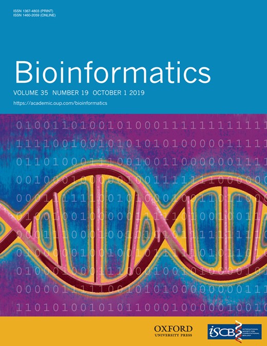
The schema of ADMM for solving NLRR

2.2 Selection of penalty coefficient of low rank

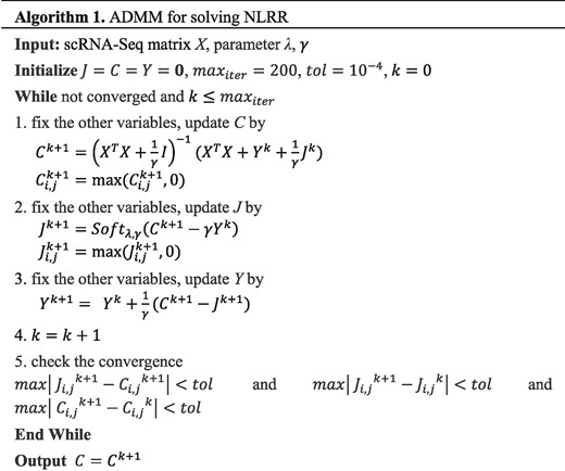
According to the schema of the optimization algorithm, there are two user-defined parameters, λ and$\mathrm{ }\gamma$⁠. In the experiments, we find the structure of learned similarity matrix is really sensitive to the selection of parameter λ. Taking the Pollen’s dataset (Pollen et al., 2014) as an example, the effect of different values of λ is shown in Figure 2.

Fig. 2.

The heatmaps of learned similarity matrix from Pollen’s dataset with (A) λ = 0.01, (B) λ = 0.7, (C) λ = 5 and (D) λ = 10. Each color in the color bar denotes a specific type of cells and the depth of color indicates the strength of similarity

Figure 2 shows that a proper value of λ would lead to a better similarity matrix corresponding to the real cell types. However, the optimal λ is distinct for different datasets. The parameter λ controls the learned similarity matrix S as follows: (i) when$\mathrm{ }\lambda \to 0$⁠, the diagonal element $S_{\mathit{ii}}$ will be close to 1 and $S_{\mathit{ij},i\ne j}$ will be close to 1, because the expression of cell can represent itself without the low-rank constraint. The form of S would be similar to Figure 2A. (ii) when$\mathrm{ }\lambda \to \infty$⁠, matrix S can be divided into one or a few blocks. For each block, the similarities in each column or row are approximately the same. That is because a very large $\lambda$ leads to a lower rank, which is similar to Figure 2D. (iii) when $\lambda$ is proper, the value of similarity in each column will look like Figure 2B.

If the parameter λ is proper, the similarities of each row (or column) in matrix S can be divided into two groups like Figure 3 shows, whose similarities in one group are larger than another one. Inspired by this characteristic, we propose an approach to select the proper λ automatically based on analyzing the locality of coefficient matrix C before constructing the similarity matrix. First, we obtain a localized similarity matrix as follows:

$$P_{\mathit{ij}}=\left\{\begin{array}{c}{C}_{\mathit{ij}}\hspace{1em}\hspace{1em}\mathrm{if} C_{\mathit{ij}}>(C_{\mathit{ii}}/f)\hfill \\ 0\hspace{1em}\hspace{1em}\hspace{1em}\mathit{Otherwise}\hfill \end{array}\mathrm{ }\right.$$

(10)

where $C$ denotes the self-similarity of cell i for a selected λ. We use $C_{\mathit{ii}}$ as a reference similarity score and retain the similarities larger than $C_{\mathit{ii}}/f$⁠. $f\mathrm{ }$is a coefficient of relaxation, which is set to 1.5 in this study.

Fig. 3.

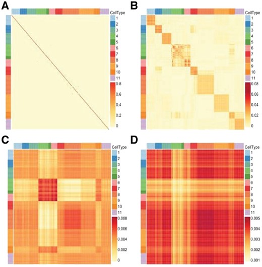
The ordered similarity of a cell in Pollen’s dataset. The similarities of cells in the yellow dashed circle are far larger than the remaining part

Based on the localized similarity matrix P, we further analyze the number of minimal neighbors (NoMN). The NoMN is defined as the minimal degree of all cells. The degree of a cell is defined as follow:

$${\mathrm{deg}}^i={\mathrm{Count}}_{\mathrm{for}\mathrm{ }\mathrm{all}\mathrm{ }j}\left(P_{\mathit{ij}}\ne 0\right)\mathrm{ }$$

(11)

$\mathrm{Count}\mathrm{ }$where ‘Count’ denotes the number of similarities satisfying the Boolean function. When we raise parameter λ gradually, the NoMN will drastically jump to a value larger than one. The parameter λ around the tipping point is selected to obtain the final similarity matrix. The detail of the analysis could be found in the Section 3.2. The final similarity is $S=P^T+P$⁠.

2.3 Spectral clustering

Spectral clustering is a popular and efficient method to cluster the points based on the similarity matrix (Von Luxburg, 2007). Spectral clustering has been applied to identify cell types successfully (Park and Zhao, 2018; Wang et al., 2017). In the proposed method, we also adopt the spectral clustering on the learned similarity matrix. The process of spectral clustering used in our method is shown in Figure 4. The details of the spectral clustering could be found in Von Luxburg (2007).

Fig. 4.

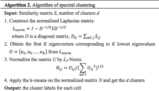
The process of spectral clustering based on the learned similarity

2.4 Framework of SinNLRR

SinNLRR contains three elementary steps, including preprocessing, similarity matrix learning and analysis. Data preprocessing is an efficient mean to reduce the noise of original data. Previous studies applied different preprocessing methods, such as gene filter (Kiselev et al., 2017; Wang et al., 2017;), imputation (Li and Li, 2018; Lin et al., 2017), dimensionality reduction (Lin et al., 2017; Pierson and Yau, 2015). In SinNLRR, we apply the gene filtering and L₂-norm as preprocessing approach. For the gene filter step, we remove the genes whose expressions (the expression of the gene is non-zero) are <5% of all cells. The L₂-norm is applied on gene expression of each cell as follows:

$${X_{\mathit{ij}}}^{\mathrm{norm}}=X_{\mathit{ij}}/\sqrt{\sum _{\mathrm{all}\mathrm{ }i}{X_{\mathit{ij}}}^2}\mathrm{ }$$

(12)

where $X_{\mathit{ij}}$ denotes the expression of gene i in cell j. L₂-norm is widely used in subspace clustering to eliminate the scale differences among samples (Vidal and Favaro, 2014). Then, SinNLRR learns the similarity matrix based self-expression learning with non-negative and low-rank constraints. The proper penalty factor λ is selected automatically based on finding the tipping point of NoMN. Finally, spectral clustering is performed on the similarity matrix to get the final clusters. Besides, the learned similarity matrix could also be used in visualizing and prioritizing gene markers. The whole framework of SinNLRR is shown in Figure 5.

Fig. 5.

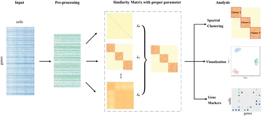
The framework of SinNLRR. SinNLRR takes the scRNA-seq expression matrix as input, and applies data preprocessing, including gene filtering and normalization. Then SinNLRR learns the proper similarity matrix by self-expression with non-negative and low rank constraints. SinNLRR could select proper penalty factor of low rank constraint automatically. The learned similarity matrix could be incorporated with spectral clustering for identifying the cell types, with t-SNE for visualization and Laplacian score for prioritizing gene markers

3 Results

3.1 Datasets

We collect 10 datasets of human and mouse scRNA-seq that involve in various tissues and different biological process such as cell development and cell differentiation. These datasets contain different scales of cells from dozens to thousands. Moreover, the datasets are derived from various single-cell RNA-seq techniques (Wu et al., 2013), such as SMARTer, Drop-seq and use different unit count, e.g. RPKM (reads per kilobase of transcript per million mapped reads), FPKM (fragments per kilobase of transcript per million mapped reads). Especially, the Lin dataset (Lin et al., 2017) is a mixed dataset, including GSE41265, GSE42268 and GSE45719 from GEO database. All the original expressions are applied with the log transformation. The detailed descriptions of the datasets are shown in Table 1.

Table 1.

The description of datasets used in experiments

Dataset	Cells	Genes	Cell types	Protocol	Units	Species
Darmanis (Darmanis et al., 2015)	420	22085	8	SMARTer	CPM	Homo sapiens
Goolam (Goolam et al., 2016)	124	40315	5	Smart-seq	CPM	Mus musculus
Lin (Lin et al., 2017)	402	9437	16	Fusion	TPM	Mus musculus
Pollen (Pollen et al., 2014)	249	14805	11	SMARTer	TPM	Homo sapiens
Usoskin (Usoskin, et al., 2015)	622	17772	4	Usoskin(2010)	RPM	Mus musculus
Treutlein (Treutlein et al., 2014)	80	959	5	SMARTer	FPKM	Mus musculus
Engel (Engel et al., 2016)	203	23337	4	Smart-seq2	TPM	Homo sapiens
Tasic (Tasic et al., 2016)	1727	5832	48	SMARTer	TPM	Mus musculus
Zeisel (Zeisel et al., 2015)	3005	4412	48	–	UMI	Mus musculus
Macosko (Macosko et al., 2015)	6418	12822	39	Drop-seq	UMI	Mus musculus

3.2 Performance metrics

To evaluate the performance of clustering methods, we select two common metrics: normalized mutual information (NMI) (Strehl and Ghosh, 2003) and adjusted rand index (ARI) (Wagner and Wagner, 2007). NMI and ARI are calculated as follows:

$$\mathrm{NMI}(T,P)=\frac{I(T,P)}{[H\left(T\right)+H\left(P\right)]/2}$$

(13)

$$\mathrm{ARI}\left(T,P\right)=\frac{{\sum }_{\mathit{ij}}\left(\genfrac{}{}{0pt}{}{n_{\mathit{ij}}}{2}\right)-\left[{\sum }_{\mathit{ij}}\left(\genfrac{}{}{0pt}{}{n_{\mathit{ij}}}{2}\right){\sum }_{\mathit{ij}}\left(\genfrac{}{}{0pt}{}{n_{\mathit{ij}}}{2}\right)\right]/\left(\genfrac{}{}{0pt}{}{n}{2}\right)\mathrm{ }}{\frac{1}{2}\left[{\sum }_i\left(\genfrac{}{}{0pt}{}{a_i}{2}\right)+{\sum }_j\left(\genfrac{}{}{0pt}{}{b_j}{2}\right)\right]-\left[{\sum }_i\left(\genfrac{}{}{0pt}{}{a_i}{2}\right){\sum }_j\left(\genfrac{}{}{0pt}{}{b_j}{2}\right)\right]/\left(\genfrac{}{}{0pt}{}{n}{2}\right)},\mathrm{ }$$

(14)

where $T=\left\{T_1,T_2\dots ,T_k\right\}$ denotes the true group of cells, and $P=\left\{P_1,P_2\dots ,P_k\right\}$ consists of the predicted groups. H denotes the entropy while $I\left(T,P\right)$ denotes the mutual information of T and P. $n_{\mathit{ij}}$ means the number of cells in both $T_i$ and $P_j$⁠, $a_i$ is the number of cells in $T_i$ while $b_i$ is the number of cells in $P_i$⁠. $\left(\genfrac{}{}{0pt}{}{n}{2}\right)=n(n-1)/2$⁠. The two metrics evaluate the similarity of predicted labels and true labels based on different theories. Previous study (Romano et al., 2016) has showed $\mathrm{NMI}$ should be selected when the numbers in reference clustering labels are unbalanced, and $\mathrm{ARI}$ otherwise. The larger value of NMI or ARI implies the better performance. In this paper, we select metrics to compare different clustering methods.

3.3 Parameter selection by NoMN

To solve the sensitivity of SinNLRR with the parameter λ, we propose the NoMN to select λ automatically. The description of NoMN can be found in Section 2.2. We increase the λ from 0 to 2 or 2.5 with interval 0.1 for datasets whose number of cells is smaller than 1000 or otherwise, respectively. The responding change of NoMN, NMI and ARI in datasets of Darmanis, Pollen and Macosko is shown in Figure 6. The NoMN jumps from 1 to a bigger value and increase quickly when λ reaches a certain point. Figure 6 shows that SinNLRR achieves the better performance when λ is around the tipping point. In practice, we determine the proper value of λ when the NoMN is larger than three for the first time for small dataset (the number of cells is smaller than 1000), and larger than one for large scale datasets. The search for the proper λ requires multi-runs of NLRR. However, NLRR can be in parallel computed, and we increase the value of λ with the increment of 0.2 to further speed the calculation up. The analysis of λ in remaining datasets and the effect of parameter $\gamma$ could be found in Supplementary Figures S1 and S2.

Fig. 6.

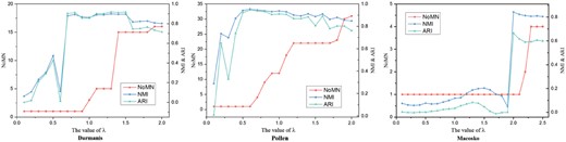
The corresponding NoMN, NMI and ARI with different values of parameter λ. The left y-axis is the value of NoMN, while right y-axis denotes the value of NMI and ARI

3.4 Comparative analysis of clustering

In this section, we apply SinNLRR on 10 scRNA-seq datasets described in Table 1. These datasets contain different scales of cells and the subtype numbers. We select five state-of-art methods, SNN-Cliq (Xu and Su, 2015), SIMLR (Wang et al., 2017), NMF (Shao and Höfer, 2017), Corr (Jiang et al., 2018) and MPSSC (Park and Zhao, 2018). In these methods, SNN-Cliq, Corr, SIMLR and MPSSC focus on calculating pairwise similarities between cells or learning the similarity from multi-kernels, and NMF identifies the cell types based on the values in the latent dimension. For fairness, we provide the true number of clusters to Corr, SIMLR, MPSSC and NMF while SNN-Cliq cannot be set to a certain number of clusters, and other parameters are set to default. We use the native spectral clustering (SC) (Von Luxburg, 2007) with Pearson similarity as a baseline method. As the algorithm Corr is time-consuming for big datasets (more than 3 days for cells larger than 1000), we abandon the results of Corr on the datasets Tasic, Zeisel and Macosko. Figure 7 summarizes the NMI and ARI of these methods on the 10 datasets. The proposed method SinNLRR gets the best performance in seven datasets based on NMI and ARI, and gets top two performances in nine datasets. Although the identification of cell types is an unsupervised problem and is complex according to different conditions, the results show the better robustness and ability of generalization of SinNLRR. Moreover, we also analyze the time complex of SinNLRR and the comparison of running times with other methods. The details can be found in Supplementary Material Section D.

Fig. 7.

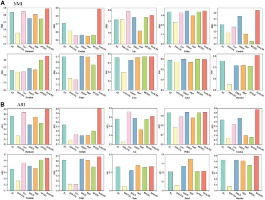
The (A) NMI and (B) ARI of SC, SNN-Cliq, Corr, SIMLR, NMF, MPSSC and SinNLRR on 10 datasets. Corr is not applied on Tasic, Zeisel and Macosko because of the time complexity

In the real biological experiment, the number of clusters is usually inaccessible, so evaluating the number of clusters is another important aspect in clustering methods. Based on the normalized Laplacian matrix L, we apply eigengap (Von Luxburg, 2007) to determine the number of cluster k by maximizing the eigenvalues gap $|{\lambda }_k-{\lambda }_{k-1}|$⁠, where ${\lambda }_1<{\lambda }_2\dots <{\lambda }_n$ is the eigenvalues of the Laplacian matrix L. This approach is also applied in SIMLR and MPSSC. SNN-Cliq and Corr also provided the methods to estimate the number of clusters. The comparison results on 10 datasets are shown in the Supplementary Table S1. Although these methods are weak to estimate the number of clusters accurately, SinNLRR could be a better selection which is closest to the true numbers.

3.5 Visualization and gene markers

Visualization of the scRNA-seq data in the lower dimensional is a powerful approach for biologists to pre-identify the subgroups of cells (Dong et al., 2018; Zhong et al., 2018). The t-distributed stochastic neighbor embedding (t-SNE) is one of the most popular tools for visualization (Maaten and Hinton, 2008). We use the similarity matrix learned by SinNLRR as the input of the modified t-SNE, which is the same with previous studies (Wang et al., 2017), to distinguish the subgroups of cells intuitively. We focus on two datasets Darmanis and Goolam described in Table 1. Darmanis dataset (Darmanis et al., 2015) is a crowd of 420 cells from the adult and fetal human brain, consisting of 62 astrocytes, 20 endothelial, 110 fetal quiescent neurons, 25 fetal_replicating neurons, 16 microglia, 131 neurons, 38 oligodendrocytes and 18 oligodendrocyte precursor cells. The second dataset is from Goolam et al. (2016). The cells in this dataset are derived from mouse embryos, including five stages of development: 2-cell (16 cells), 4-cell (64 cells), 8-cell (32 cells), 16-cell (6 cells) and 32-cell (6 cells). We select the native t-SNE, and similarity matrix based on SIMLR and MPSSC as comparison methods. It should be noted that SIMLR and MPSSC need the true cluster number to learn the similarity matrix, while native t-SNE and SinNLRR don’t, so we use the estimated cluster number instead. The two-dimensional t-SNE plots of two datasets are shown in Figure 8. In Figure 8A, SinNLRR groups the same type of cells better overall. The groups of SIMLR are more compact because of its block structure, but it divides the fetal quiescent neurons and neurons into a few subgroups. All the visualizations based on the learned similarity matrices are better than native t-SNE. As seen in Figure 8B, SinNLRR performs better in Goolam dataset.

Fig. 8.

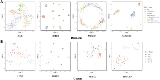
Visualization of the cells in (A) Darmanis dataset and (B) Goolam dataset based on the native t-SNE and modified t-SNE with learned similarity matrix from SIMLR, MPSSC and SinNLRR

The learned cell-to-cell similarity matrix can be further applied to identify the gene markers in each type of cells. We perform the bootstrapped Laplacian score proposed by Wang et al. (2017) on the similarity matrices of Darmanis and Goolam datasets. We select top 10 gene markers of the two datasets, and present the average of log transformed counts and sparsity (the proportion of non-zero expressed cells) in each cell type. The results are shown in Figure 9. In Darmanis dataset, the selected top 10 genes are in agreement with previous studies. The genes AGXT2L1, AQP4, FGFR3 and GJA1 are highly expressed in astrocytes and had been recognized as gene markers, while Opalin and ERMN are oligodendrocytes-specific genes related to the novel transmembrane proteins (Cahoy et al., 2008; Darmanis et al., 2015; Oldham et al., 2008). Especially, FGFR3 and AQP4 act as the important receptors for early astrocyte development. Popson et al. (2014) had identified IFITM1 as a pan-endothelial marker of endothelial cells in the bladder, brain and stomach. STMN2 is a neuron-specific gene both in adult and fetal neurons, and SOX11 is the enriched gene in fetal neurons (Darmanis et al., 2015). In Goolam dataset, OMT2A, OMT2B and OOG1 had been reported as the potential stage-specific genes (Tang et al., 2010). KLF17 was validated to highly expresses in earlier stages of development and was absent in blastocysts (Blakeley et al., 2015) and BTG4 showed the declining trend of expression in early mouse embryos (Yu et al., 2016). OBOX8 was found to express highly around 4-cell stage. APELA, B020004C17rik, EXOC3L2 and PPP1R16B are the novel potential gene markers.

Fig. 9.

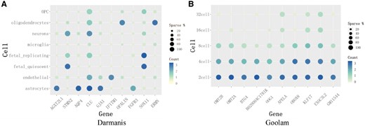
The top 10 gene marker in (A) Darmanis and (B) Goolam datasets. The x-axis is the gene name while y-axis is the cell types. The color denotes the expression level of genes and the size of the circles denotes the sparsity of the genes expressing in cells

4 Discussion

Identification of the cell types based on scRNA-seq data is one of the basic issues in Human Cell Atlas project (Rozenblatt-Rosen et al., 2017). However, the scRNA-seq data contains high noise and dropouts, which bring great challenges for clustering. In this paper, we have proposed a novel similarity based clustering method, called SinNLRR. SinNLRR is motivated by the self-expression among cells in the same type and assumes the non-negative and low-rank characteristics of the similarity matrix.

SinNLRR exposes global and robust similarity structures than the traditional pairwise similarity metric, such as Pearson correlation or Gaussian kernel. We apply the ADMM to solve the corresponding convex problem and define the NoMN to select the proper penalty factor. The learned similarity matrix could be incorporated with spectral clustering for grouping cells, t-SNE for visualization and Laplacian score for selecting gene markers. We evaluate the performance of SinNLRR on scRNA-seq datasets derived by different single-cell techniques and scales and find SinNLRR achieves more robust and accurate results than other state-of-the-art methods. In additional, SinNLRR could be useful in other applications of scRNA-seq analysis, such as pseudo-time reconstruction (Ji and Ji et al., 2016) and potency measure of cells (Guo et al., 2017; Shi et al., 2018), which require the clustering results or the cell-to-cell networks as a preliminary process.

Besides, several available biological information, such as protein–protein interaction networks and subcellular localization (Li et al., 2019), provides a lot of auxiliary information, which is helpful in gene selection and data imputation while gene regulatory networks (Li et al., 2017; Zheng et al., 2018) present a biological interpretation of cell states. It is promising to incorporate SinNLRR with these data to further enhance the performance. Currently, SinNLRR can handle the datasets with thousand cells in a reasonable time. However, designing the version for really large scale scRNA-seq would be one the of directions in the future researches.

Funding

This work was supported in part by the National Natural Science Foundation of China [61832019, 61622213], the 111 Project (No. B18059); the Hunan Provincial Science and Technology Program [2018WK4001]; and the Fundamental Research Funds for the Central Universities of Central South University [No.2018zzts028].

Conflict of Interest: none declared.