DECO: decompose heterogeneous population cohorts for patient stratification and discovery of sample biomarkers using omic data profiling

Abstract

Motivation

Patient and sample diversity is one of the main challenges when dealing with clinical cohorts in biomedical genomics studies. During last decade, several methods have been developed to identify biomarkers assigned to specific individuals or subtypes of samples. However, current methods still fail to discover markers in complex scenarios where heterogeneity or hidden phenotypical factors are present. Here, we propose a method to analyze and understand heterogeneous data avoiding classical normalization approaches of reducing or removing variation.

Results

DEcomposing heterogeneous Cohorts using Omic data profiling (DECO) is a method to find significant association among biological features (biomarkers) and samples (individuals) analyzing large-scale omic data. The method identifies and categorizes biomarkers of specific phenotypic conditions based on a recurrent differential analysis integrated with a non-symmetrical correspondence analysis. DECO integrates both omic data dispersion and predictor–response relationship from non-symmetrical correspondence analysis in a unique statistic (called h-statistic), allowing the identification of closely related sample categories within complex cohorts. The performance is demonstrated using simulated data and five experimental transcriptomic datasets, and comparing to seven other methods. We show DECO greatly enhances the discovery and subtle identification of biomarkers, making it especially suited for deep and accurate patient stratification.

Availability and implementation

DECO is freely available as an R package (including a practical vignette) at Bioconductor repository (http://bioconductor.org/packages/deco/).

Supplementary information

Supplementary data are available at Bioinformatics online.

1 Introduction

The areas of precision medicine and big data analysis are growing exponentially along this decade, driven by the hope to improve molecular characterization of diseases and patient diagnosis and treatment based on the extensive use of omic data (i.e. data produced by genomic, transcriptomic and proteomic techniques). Collecting information from large sample populations is also a main aim of many biomedical projects to allow comprehensive studies that include many patients with all types and subtypes of the studied disease (Ashley, 2016). Most of the times, however, collecting a huge amount of data make analyses noisy, and bring the need to delve inside data, applying different filtering techniques or attempting to remove irrelevant information: trying to change from extensive big data to informative smart data. Such accumulation of large-scale data creates a complexity that combined with sample variability gives rise to a difficult scenario, where it is easy to make mistakes when searching for novel specific markers. In this sense, individual variability is one of the most intricate issues to deal with in biomedical studies of large patient cohorts (De Palma and Hanahan, 2012; Rodriguez-Gonzalez et al., 2013).

Currently, omic techniques applied to clinical and biomedical studies are generating large-scale molecular profiles from patients. One of the omic techniques that has provided best and broader results is genome-wide expression profiling. Changes in gene expression among disease subtypes are detectable using robust differential expression (DE) methods, like T-test, Mann–Whitney–Wilcoxon, SAM (Tusher et al., 2001) and LIMMA (Smyth, 2004), which have been applied successfully in the last decade in group-versus-group comparisons. However, while these approaches have been applied expecting differences between two pre-defined categories of samples, the clinical data from patients exhibits considerable variability unrelated to the aim of study. This problem is even larger if we compare closely related pathological disease subtypes, where subtle differences can mark dramatic changes in diagnosis and prognosis. Besides this patient heterogeneity, cancer-related studies may also show intra-tumour variability corresponding to the alteration of tumour cells related to the microenvironment, evolving mutations or longitudinal changes along the progression of the disease (Bedard et al., 2013). Consequently, the big impact of individual heterogeneity on biomedical omic studies makes finding specific and reproducible gene markers highly challenging (Gillies et al., 2012).

Intra-tumour heterogeneity could result in abnormal gene expression of a subset of genes. This idea that genes are often deregulated in only a subset of patients, especially in cancer studies, led to the development of an interesting method called Cancer Outlier Profile Analysis (COPA) (MacDonald and Ghosh, 2006). Outlier genes are intended to show aberrant expression levels only in a subset of tumour or case samples as a consequence of the genotype. Indeed, the difference between an outlier and a typical differentially expressed gene (DEg) is that the outlier has a modified expression only in a minority of the studied samples, indicating a heterogeneous behaviour in such sample subset (MacDonald and Ghosh, 2006). In order to find outlier genes, several algorithms have been proposed in the last two decades. These methods are based on different modifications of statistical tests, clustering or sampling techniques applied to either original omic data or multidimensional transformed data (de Ronde et al., 2013; Li et al., 2007; Lian, 2008; Nabavi et al., 2016; Noto et al., 2015; Tibshirani and Hastie, 2007; Wang and Rekaya, 2010; Wu, 2007; Yang and Yang, 2013).

Most of these methods proposed the discovery of up-regulation events for a subset of samples when gene expression levels (mRNA) of cancer samples are compared to control samples. In the original publication of COPA, the authors attributed these differential events (DEs) to genomic translocations of DNA, a very common incident in tumour cells. Particularly, this study was focussed on prostate cancer and the fusion of TMPRSS2 and ETS transcription factor genes (Tomlins et al., 2005).

In the singular biological context of cancer, the genomic translocation is one of the many existing sources of biological heterogeneity of tumour cells (Hogenbirk et al., 2016). As mentioned before, individual genotype and phenotypical circumstances, spatial and temporal clonal evolution of tumour cells (even more pivotal if solid tumour) and technical variability (from any high or low-throughput technique) also contribute to a complex scenario where the identification of any relevant source of heterogeneity makes crucial the development of comprehensive approaches (Allott et al., 2016, Rubben and Araujo, 2017). However, we mentioned before that most of the current omic analyses focus on supervised comparisons (reference samples against case samples) which do not take into consideration these issues. For this reason, we hypothesized a four model-type scheme of possible heterogeneous profiles when two categories of samples are compared (Fig. 1), which considers typical major changes and also minor or outlier changes between classes.

Fig. 1.

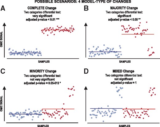
Theoretical framework presenting several types of change that include samples heterogeneity in different proportions and outliers. Four model-types of change can be expected when comparing two pre-defined classes: (A) complete change; (B) majority change; (C) minority change and (D) mixed change. The changes are shown in each model-type for a measured variable (i.e. for the specific signal of one measured omic feature, like the expression of one gene). The plots represent in blue the signal of such feature for the control samples and in red the signal of such feature for the case samples

Therefore, attending to a single omic feature profile, we could categorize the differential profiles between two classes of samples (cases versus controls) in four possible types or cases (schematic presented in Fig. 1). These possible situations are: (i) (Fig. 1A) when the feature shows a clear and complete change in all sample cases versus controls (therefore, using a standard differential test approach gives a very significant P-value <0.01***); (ii) (Fig. 1B) when the feature shows a change in the majority of the cases and, using a standard differential test approach, it will give a significant P-value (<0.05**); (iii) (Fig. 1C) when the feature shows a change only in a minority of the cases and, so, using a standard differential test may give a marginal P-value not significant (≈0.05–0.15*); (iv) (Fig. 1D) when the feature shows a significant intra-category change in both the cases and controls (mixed change) but, in this situation, the comparison between cases and controls does not give any significant change (P-value ≈1.0).

Noteworthy, the mixed changes cannot be detected by comparison of pre-determined classes. Although these mixed changes are not directly related to the design of the comparison, the consideration of them may be useful: (i) to improve the discovery of new subclasses of samples within a whole dataset (improving intra-category stratification); or (ii) to identify possible confounding phenotypic factors which are not known a priori. Therefore, these mixed changes are not directly related to pre-defined classes, since they contain the same changes in these classes.

Motivated by these differential scenarios described in Figure 1, we have developed in R a bioinformatic algorithm called DEcomposing heterogeneous Cohorts by Omic data profiling (DECO) to identify and categorize features that mark differences between closely related biological states. Our method includes first a stratified combinatorial sampling without replacement [that we called recurrent differential analysis (RDA)] to select multiple sample subsets in the following types of comparisons: (i) two pre-defined categories (supervised binary analysis); (ii) more than two categories of samples (multiclass analysis); (iii) and not pre-defined classes (unsupervised analysis). Sampling approaches have demonstrated high stability rates in the feature selection procedure (Baty et al., 2008; Verma et al., 2014), also using empirical Bayesian methodologies (Qiu et al., 2006). Thus, the proposed sampling enables an agnostic exploration of differential signatures and allows analysis of complex situations. For example, situations when the variability among individuals is not related to the main pre-defined phenotypic classes; when there are possible errors in the class assigned to some individuals; or when there are some features which only change in a subset of samples but in the same proportion in cases and controls.

After the differential analysis, the method applies non-symmetric correspondence analysis (NSCA) (Lauro and D’Ambra, 1984) to integrate a predictor-response directional information between samples and features. The details of the new algorithm are presented in the following sections, including a full description of the methodology and an extensive comparison of the performance with seven other methods designed to analyze differences and find heterogeneity and outliers in disease sample cohorts. The method is tested using 2 simulated datasets and 5 different sets of omic data from clinical cohorts, 2 of which include several 100 samples.

2 Materials and methods

2.1 DECO algorithm

The developed method includes six main steps that are essentially described below point by point. The developed method includes six main steps that are essentially described below point by point. For more technical purposes, a complete detailed description of the algorithm is included in Supplementary Material S1. At the end of this Supplementary Material, we also include a Supplementary Figure S1 that presents a schematic view step by step of the workflow of the method.

2.1.1 Step 1

Starting from an omic data matrix (composed of m features and n samples), DECO is initiated by applying the subsampling procedure (called RDA) to identify, select and rank all significant changes found for any feature (e.g. any gene) between two subsets of samples. The size of the subsets is indicated by the user (being by default a minimum of three samples per subset) (Babu, 1992). The two subsets of samples are generated randomly by selecting all possible subsets of the fixed size (i.e. 3×2) from the whole sample set. In this way, the method produces many iterative contrasts for each feature. The sample set can be grouped according to the input information provided by the user (i.e. grouped into classes of samples if it is a supervised analysis, or without pre-defined categories if it is unsupervised). All the differential contrasts are done using the eBayes method from LIMMA (Smyth, 2004). Once all significant changes are obtained, they are saved in a big table including all the P-values per sample subset per feature. Then, these P-values are summarized in a unique score (S_f) per feature, using the Fisher’s method for combined probability. In other words, to combine the probabilities after all the significant iterations (R) that pass a pre-defined threshold (by default: adjusted P-value <0.01), the method calculates the S_f score applying the Fisher’s method and using the non-adjusted raw P-values obtained for each feature (Fisher, 1925). This combination of P-values follows a Chi-square distribution with 2 R degrees of freedom. The S_f score provides a measure of differential consistency along the subsampling procedure. Additionally, DECO generates a frequency table counting the significant differences (i.e. the DEs) where each feature and sample participates (using the threshold of significance indicated: adjusted P-value <0.01). This frequency matrix or incidence matrix (A) that adds up all the DEs (counting the number of times that each feature was significant in a given sample) is a main output of this RDA step, and it is used in the next steps of the algorithm.

2.1.2 Step 2

In the second step of the algorithm, DECO applies a non-symmetrical correspondence analysis (NSCA) on the frequency matrix (A). NSCA allows to establish an asymmetric association among features and samples in a common dimensional space transforming the frequency matrix into a matrix of centred column profiles (where the columns are the samples). We internally called this matrix Y, and it is only an intermediate element of the process. This Y matrix is used as input for an isometric factorization of the samples by Singular Value Decomposition, which decomposes all inertia or variability of Y matrix, calculating the row and column coordinates (i.e. feature and sample coordinates) from the inertia decomposition based on the Goodman’s–Kruskal τ (tau) index (Goodman and Kruskal, 1959). This decomposition generates a common n-dimensional space, where the association among features and samples can be quantify by the inner product (p) between every feature and sample coordinates (Light and Margolin, 1971; Beh and Lombardo, 2014). Thereby, the final output of this NSCA step is both the column and row profile coordinates for samples and features, that is used in the next step to calculate the inner product matrix (P).

2.1.3 Step 3

In a third step, DECO integrates, in a unique statistic [called heterogeneity statistic (h-statistic)], both the predictor-response information given by the inner product matrix (P), and the data dispersion given by a raw omic dispersion matrix (D). The inner product matrix (P) measures the strength of the asymmetric association, indicating that the higher the inner product is, the more dependency of a differential signal of a feature from the presence of certain samples is. Additionally, the omic dispersion matrix (D) measures the difference of every sample to the mean signal per feature, and it is calculated using the original omic data. The integration of D and P is detailed in Supplementary Material S1 and leads to the calculation of the newly proposed h-statistic. Given a feature and sample, this h-statistic was intended to unify the measured difference from population by the omic technique (provided by D) and the relevance of this measure in a predictor-response context among samples and features (provide by P) (Hartigan and Wong 1979). Consequently, the agreement for high values of both D and P would drive to higher values of the h-statistic. As a final result of this step, DECO would generate a matrix H including the h-statistic per feature per sample.

For a better conceptual understanding of this Step 3, it is important to mention that the inner product (P) reflects the predictor-response relationship between columns (samples) and rows profiles (features) from NSCA coordinates, while the dispersion matrix (D) provides a direct measure of the real dispersion of each sample from the mean signal per feature. The h-statistic unites both parameters, providing higher absolute values (i.e. higher positive or negative h values) when there is a concordance: (i) in the predictor-response behaviour (P) of the sample-feature tandem; and (ii) in the change of omic data (D) for the same sample and feature tandem. Throughout this paper, we demonstrate the power and suitability of this h-statistic as a replacement of raw simple omic data (such as genome-wide expression data) for classification and stratification of samples (improving the clustering properties), as well as, for the identification of new features (i.e. genes) as clear biomarkers of specific states.

2.1.4 Step 4

Once the new h-statistic is calculated, DECO applies a hierarchical bi-clustering on this H matrix instead of using the original omic data matrix. Here, the method uses Pearson correlation as distance metric and an iterative procedure based on Pearson version of Hubert’s γ coefficient to obtain the best number of different subgroups from sample’s hierarchical clustering.

2.1.5 Step 5

To identify the different types of changes described in Figure 1 (and considering the most frequent case when two categories of samples are compared), DECO calculates the overlap of omic signal between the sample’s categories, using each distribution of omic values per category. This measure is called overlap (o_f) and allows to define every feature belonging to each hypothesized four model-types of change: change complete (Fig. 1A), change in a majority (Fig. 1B), change in a minority (Fig. 1C) and mixed change (Fig. 1D).

2.1.6 Step 6

Finally, in the last step of the method, DECO ranks all features obtained based on the three main statistics mentioned above: (i) S_f score, which highlights the most significant changes from RDA; (ii) h-statistic range per feature, which indicates how discriminant each feature is, given the subclasses found by DECO; and (iii) o_f overlap plus the standard deviation of raw omic signal in each differential feature.

The performance of DECO algorithm was evaluated in comparison with seven other methods that analyze differences to find heterogeneity and outliers: COPA (MacDonald and Ghosh, 2006), OS (Tibshirani and Hastie, 2007), ORT (Wu, 2007), MOST (Lian, 2008), LSOSS (Wang and Rekaya, 2010), DIDS (de Ronde et al., 2013) and the standard t-Test (Table 1). The method is designed to support any type of omic feature properly normalized. In this work, we use genome-wide expression datasets; some obtained with high-density microarrays and other with RNA sequencing (RNA-seq). Transcriptomic is the most frequent omic data produced and present in many public repositories (e.g. GEO: https://www.ncbi.nlm.nih.gov/geo/).

Table 1.

Methods included in the benchmark

Method	Strategy	Down-regulated features	Weights size of outlier	Sample sub-group finding	Reference
COPA	Percentile—MAD	No	No	No	MacDonald and Ghosh (2006)
OS	Quantile ordered & cut-off	No	No	No	Tibshirani and Hastie (2007)
ORT	Robust t-statistic	Yes	No	No	Wu (2007)
MOST	Maximum ordered	Yes	No	No	Lian (2008)
LSOSS	Least sum of ordered subset square t-statistic	Yes	No	No	Wang and Rekaya (2010)
DIDS	Maximum value from control group	Yes	Yes	No	de Ronde et al. (2013)
DECO	RDA & NSCA	Yes	Yes	Yes	Present work (2019)

Note: Brief description of the characteristics of the computational methods to find outliers and heterogeneity that are compared in this work including their references.

2.2 Benchmark using simulated data

Simulated datasets were designed to have an expression matrix that included signals for 1100 genes and 40 samples in two classes: n₁ = 20 controls and n₂ = 20 cases (Khondoker et al., 2010). This design followed a similar scenario to the LSOSS benchmark (Verma et al., 2014), representing two different situations: (A) a dataset that included 100 genes (10%) with DE within a subset of ‘case’ samples (5 in 20) (Fig. 2A); (B) a dataset that included 100 DE genes (10%) within a subset of both ‘case’ and ‘control’ samples (5 in 20), so that there is not global DE between classes for these genes (Fig. 2B). These two scenarios correspond to balanced situations, where the number of cases and controls is the same (n₁ = n₂ = 20).

Fig. 2.

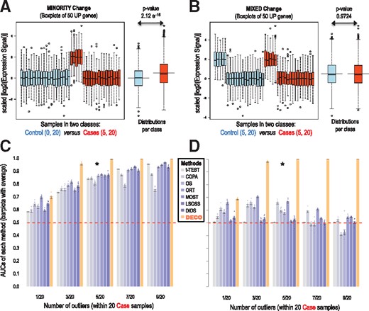
Comparison of eight methods (t-Test, COPA, OS, ORT, MOST, LSOSS, DID, and DECO) used to find significant changes that occur in a minority of samples (≈25%) and in a small proportion of features (≈10%). The analyses are done in two simulated datasets that include: 20 ‘case’ samples versus 20 ‘control’ samples and a set of 1100 genes including 100 DEg. (A) and (B): boxplots of the expression signal (in log2) along 40 samples of 50 genes that are UP-regulated. (C) and (D): barplots with the values of the average AUCs obtained using eight different methods applied to search for differential expressed genes. Each panel (C and D) includes the eight methods compared in five conditions that correspond to an increasing number of samples that had DEg: from only one sample in 20 case samples (that means a 5% of the samples affected) to 9 in 20 (i.e. a 45% of the samples affected). Plots (A) and (C) correspond to the first simulated dataset was the DEg only occur in the cases. Plots (B) and (D) correspond to the second simulated dataset was the DEg occur both in the cases and in the controls. In this way, the 100 DEg are distributed: 50 genes UP and 50 DOWN in 25% of the cases for plot (A) (that corresponds to AUCs marked with *5/20=25% in plot C); 50 genes UP and 50 DOWN in both 25% of the controls and the cases for plot (B) (that corresponds to AUCs marked with *5/20=25% in plot D). The ROC curves were calculated as true positive rates versus false positive rates. Each AUC was calculated 10 times using different simulated data matrices (error bars are included)

The true positive rate and false positive rate were calculated for each tested method using the dataset described above. The ROC curves for each method were built and the area under the ROC curves (AUCs) calculated. Each panel (Fig. 2C and D) includes the eight methods compared in five conditions that correspond to an increasing number of samples that had differential expression.

2.3 Benchmark using experimental data

To complement the results obtained with simulated data, five experimental sets of transcriptomic data corresponding to clinical cohorts from different sources, platforms and cell types were used (described in Table 2). To evaluate the results obtained from the different methods, three tests were used: GlobalTest; Principal Component Analysis (PCA) (Mardia et al., 1979) and Support Vector Machine (SVM). The details about these tests are included in Supplementary Material S1 that also includes description of the methods used (Risueño et al., 2010; Law et al., 2014).

Table 2.

Datasets for assessing DECO in comparison with other methods

Disease	Tissue	Platform	Number of samples	Normalization	Subtypes	Type of testing	Control	Case	Reference
Osteosarcoma OSC	Tumour biopsy	Affymetrix Human Gene 1.0	21	RMA	Metastasis, no-metastasis	Supervised (two classes)	Non-metastatic primary tumour	Metastatic primary tumour	bioinfow.dep.usal.es/ osteosarcoma/
Myelodysplastic syndrome MDS-1	Bone marrow CD34+ Cells	Affymetrix Human GenomeU133 Plus2.0	41	RMA	RAEB1-MDS, RAEB2-MDS	Supervised (two classes)	RAEB1	RAEB2	GSE19429 (GEO)
Myelodysplastic syndrome MDS-2	Bone marrow mononuclear cells (MNCs)	Affymetrix Human GenomeU133 Plus2.0	24	RMA	No leukaemia, low-risk MDS	Supervised (two classes)	No leukaemia	Low-risk MDS	GSE13159 (GEO) (MILE study)
Breast cancer BCC-1	Tumour biopsy	Affymetrix Human GenomeU133A	285	RMA	PAM50 (Basal, HER2+, Lum A & B)	Unsupervised (multiple classes)	—	—	GSE25055 (GEO) (GEO database)
Breast cancer BCC-2	ID-BCC and IL-BCC	Illumina HiSeq	596	log2(RPKM+1)	PAM50 (Basal, HER2+, Lum A & B)ID, IL-BCC	Unsupervised (multiple classes)	—	—	CELL (Ciriello et al., 2015)

Note: Experimental datasets used in this work to assess different computational methods to find outliers and heterogeneity.

2.4 R package and vignette

The method DECO has been fully developed in R. To facilitate open access and use, an R package called deco has been produced and it is available on Bioconductor (https://bioconductor.org/packages/deco/) (release 3.9). The package includes a detailed tutorial vignette with all the information about how to use the method.

3 Results

3.1 DECO compared to seven methods to find changes in minorities

Figure 2 shows the results of the comparisons of multiple simulated transcriptomic datasets built in the following simulations: (i) the first sets include changes that only occur in a ‘minority’ of the sample ‘cases’ but not in the ‘controls’ (Fig. 2A), with different percentages of changed genes, from 5% (1 in 20) to 45% (9 in 20) (Fig. 2C); (ii) second sets include ‘mixed’ changes occurring both in ‘cases’ and ‘controls’ (Fig. 2B), also with different percentages of changed genes from 5% (1/20) to 45% (9/20) (Fig. 2D).

We compared the AUCs in comparison to other seven methods for outlier profile detection, concluding that DECO provided the best performance for both ‘minority’ and ‘mixed’ changes (Fig. 2C and D). As shown, the increment in outlier samples from 5 to 45% leads to better results for all the methods (Fig. 2C). It is clear that the most difficult case for all the methods is the condition when only one outlier (i.e. 1 out of 20 samples) is present and also when the type of change is ‘mixed’. This scenario corresponds to first barplots in Figure 2D, in condition 1/20, where AUCs are all close to 0.50 (similar to random). The improvement provided by DECO is clear in these ‘mixed’ cases when the number of outliers increases (Fig. 2D), showing that all the other methods rely in the expectation that the control samples should not suffer anomalous changes. Additionally, these figures reveal that DECO achieves a very good performance (AUC > 0.90) with at least three outlier samples. The results indicate the initial hypothesis of stable expression profile along the control category is essential for all the other methods tested.

3.2 Detection of changes in different sample subsets in a large-scale dataset

To gain insights in how DECO responds on a large omic dataset with changes in a small proportion of genes, we built another transcriptomic simulated set: 40 samples and 10 000 genes, including only 250 genes presenting significant changes (2.5% DEg) (Fig. 3A). These differential features followed five distinct profiles, similar to the ones described in Figure 1, each containing 50 genes: (i) two profiles (p1, p2) of 50 genes showing ‘complete’ change in all cases versus controls (UP-regulated in controls, p1, or DOWN-regulated in controls, p2); (ii) two profiles (p3, p4) of 50 genes showing changes in a ‘minority’ (25%) of the samples, either in the cases or the controls (UP-regulated in five controls, p3, or UP-regulated in five cases, p4); (iii) one profile (p5) of 50 genes showing a ‘mixed’ change in a 25% of the samples (5/20) in both categories: controls and cases. The heatmap placed as Figure 3A presents these profiles within the whole set of 10 000 genes, corresponding to the expression data matrix.

Fig. 3.

Analysis of a large simulated dataset that includes 20 cases versus 20 controls measuring 10 000 genes, where 250 genes had a significant differential expression change in different subsets of the samples. (A): heatmap of the full expression matrix including the 40 samples and all the 10 000 genes. (B): heatmap of the expression of the 40 samples and 112 genes (DEg) that LIMMA method found as differentially expressed. (C): heatmap of the expression of the 40 samples and 249 DEg that RDA method found. (D): heatmap plotting the h-statistic of the 40 samples and 249 DEg that DECO method (RDA+NSCA) found. The dataset includes six different sample subsets that were found by DECO and characterized according to their gene profiles in six ‘subclasses’ [c1, 2, 3, 4, 5, 6]. The specific gene ‘profiles’ identified were: [p1] profile including 50 genes UP in all controls with respect to the cases; [p2] profile including 50 genes DOWN in all controls with respect to the cases; [p3] profile including 50 UP only in 5 controls; [p4] profile including 50 UP only in 5 cases; [p5] profile including 50 UP in both 5 cases and 5 controls (5/2=25%)

We run SAM and LIMMA, two well-established and commonly-used methods for differential expression analysis (Smyth, 2004; Tusher et al., 2001), on the expression data matrix described above (using adjusted P-value ≤0.05). These methods were expected to find at least all features corresponding to ‘complete’ changes between categories (i.e. the 100 genes included in profiles p1 and p2). SAM did it correctly, while LIMMA found 112 significant DEgs (Fig. 3B). These genes were: 95 with ‘complete’ change profile (84.8%), 11 with ‘minority’ change profile (9.8%) and 5 genes that really did not have differential expression change (i.e. 4.4% false positives) (Fig. 3B).

We also run DECO on the same data matrix and the results are shown in two steps in Figure 3C and D. First, the RDA step selected the most significant changes identifying 249/250 true positive features. Figure 3C presents the result in a heatmap and a hierarchical clustering using the raw expression signal of these 249 genes selected by DECO. As it can be seen, the genes are arranged in five different feature profiles (p1, 2, 3, 4, 5) and the samples are correctly classified in six subclasses (c1, 2, 3, 4, 5, 6) according to their corresponding profiles (Fig. 3C). These subclasses could not have been found through just applying LIMMA (Fig. 3B), the features selected by LIMMA only separated the main known classes (cases and control), and one case sample was misclassified (see clustering in Fig. 3B).

Despite the correct classification of the genes in five profiles and the samples in six subclasses obtained using the raw expression signal with RDA, the sample’s dendrogram (Fig. 3C) indicated that one of the subclasses (c6) did not have a distinct expression profile from the global matrix (Fig. 3A). This subclass has values that represent small variations from the mean expression signal of the whole dataset. Thus, the samples within subclass c6 were poorly defined for a future prediction. Alternatively, Figure 3D shows a heatmap built with the h-statistic matrix, derived from running DECO, instead the original omic matrix. The h-statistic improves subclasses separation, giving more defined profiles to the selected features and the samples. Thus, c6 subclass is now defined by an increment of p2 profile and a decrease of p1 profile. Moreover, c1 and c4 subclasses show now a differential signal that comes from the ‘complete’ profiles (p1 and p2, respectively) plus another differential signal that comes from the ‘mixed’ profile (p5) (Fig. 3D). These sample profiles are not well identified using the expression signal, showing that the h-statistic provided by DECO is more accurate for the characterization and stratification of samples.

3.3 Finding differences in absence of global changes: tests on three clinical datasets

To compare the method with other approaches in a real scenario, we selected three experimental datasets derived from clinical studies done in collaboration with biomedical groups. After applying SAM and LIMMA, each dataset did not show any significant difference in the comparison of two subtypes of patients (adjusted P-value <0.05) (Fig. 4A). The three datasets (see Table 2) and the group-versus-group comparisons were: (i) an osteosarcoma dataset (OSC) including samples of primary tumour biopsies from 21 patients that were treated in the same way, where some of them (n = 12) never developed metastasis after treatment but others (n = 9) suffered metastasis from the primary tumour; (ii) a myelodysplastic syndrome dataset (MDS-1) of CD34+ selected cells from bone marrow of 41 patients suffering two closely related MDS subtypes (RAEB1 n = 21 and RAEB2 n = 20); (iii) other MDS-2 of mononuclear cells from bone marrow of donors that usually had anaemia but not dysplasia (n = 11) and patients with low-risk MDS (n = 13). It is important to mention that the stratification of MDS is challenging, especially, when it is based on gene expression profiling (Zeidan et al., 2014).

Fig. 4.

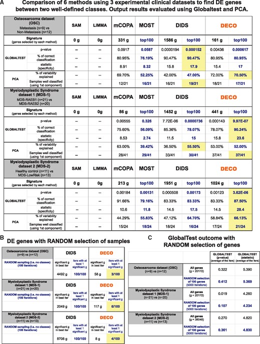
Results of the comparison of six methods (SAM. LIMMA, mCOPA, MOST, DIDS and DECO) applied to find differential expression signal in three distinct experimental datasets derived from clinical studies: OSC including 21 samples from primary tumours, 12 that never had metastasis after treatment and 9 that suffered metastasis (the comparison is done: metastatic tumours versus non-metastatic tumours); MDS-1 of CD34+ selected cells from bone marrow from 41 patients suffering two closely related MDS subtypes (RAEB1 n=21 and RAEB2 n=20); MDS-2, another MSD of mononuclear cells from bone marrow of donors that did not have any kind of dysplasia or leukaemia (n=11) and patients with that had a low-risk MDS subtype (n=13). The number of DEg found by each method is indicated below the name of the method for each dataset. Two statistical tests (GlobalTest and PCA, see Section 2) are run to evaluate the value of the genes found by each method. Yellow boxes indicate the best results for the parameters measured with GlobalTest and PCA (A). Panel (B) shows the number of significant genes found with DIDS or DECO methods in each of the three experimental datasets when samples in the two classes are assigned randomly. The comparison is done 100 times and all genes that are found in these 100 iters are indicated, as well as the number of iters that gave at least one significant gene (e.g. for the OSC dataset: 100/100 in the case of DIDS and 3/100 in the case of DECO). Panel (C) shows the values of the parameters that GlobalTest gave with each dataset when all the genes of the expression data matrix are selected as the input to the test or when 100 genes are selected randomly. This information provides a random control for the value of GlobalTest parameters.©

As indicated above, the pairwise comparison to find differences, using SAM and LIMMA, of the groups described in these three datasets did not identify any gene with a significant change (Fig. 4A). Since these standard methods for differential expression analysis applied to these clinical datasets did not reveal any differences, we tried DECO and other methods better suited to discover subtle differences. Based on previous studies that compared COPA, OS, ORT, MOST and LSOSS methods for cancer outlier discovery (Karrila et al., 2011), we considered MOST as the best of them for different scenarios and used it for these comparisons. Additionally, mCOPA (Wang et al., 2012) and DIDS (de Ronde et al., 2013) were also included in this experimental benchmark because their capability to find outlier genes had been well reported. As described in Section 2, two independent tests (GlobalTest and PCA) were used to assess the relevance of the set of significant genes found by each method (Fig. 4A). The number of selected genes (e.g. OSC: 331 genes using mCOPA, 1586 DIDS and 161 DECO) was the number found as significant (P-value ≤0.05) according to the respective algorithm.

The results obtained for each clinical dataset are presented in an illustrated table in Figure 4A. As mentioned, none of the well-established methods were able to find differential genes between the two categories of samples defined in each dataset. Furthermore, the other methods applied (mCOPA, MOST, DIDS and DECO) showed a great difference in the number of gene changes found. DIDS always provided by far the largest list, selecting 10 times more genes than DECO in the case of the OSC. It is clear that it is not easy to compare the value of the gene sets found by each method if they are very different in size. For this reason, we run the tests using only the top 100 genes with best P-values provided by each method (mCOPA did not provide a gene rank). We observed that DECO gave best results for the two datasets of myelodysplasia (MDS-1 and MDS-2, Fig. 4A) and a close result to DIDS for the OSC. Globaltest is a response-outcome test that allows determining how a given gene set marks the difference between two sample categories compared (i.e. the gene set provided by each method was used in Globaltest as a priori input group of tested variables) (Goeman et al., 2004). Based on the evaluation using Globaltest, the top 100 signature of DECO gave the best P-values: better than MOST in all cases and better than DIDS in the case of MDS-1 and MDS-2. Additionally, the PCA results agree with Globaltest, indicating that the gene sets provided by DECO assign better the samples to their expected category in the MDS cases. Only in the case of osteosarcoma, DIDS seems to be slightly better. To validate these results, we repeated the differential expression analyses doing a random selection of samples in the two categories and evaluating how many significant genes were found in 100 iterations by the algorithm DECO or by the other method that sometimes performed better (i.e. DIDS). These random tests showed that DIDS gave many false positives, selecting many more significant genes that should not be found in a random model (Fig. 4B). The robustness of the Globaltest was also validated using a random selection of 100 genes in 5000 iterations for each dataset and showing that the resulting P-values were never significant (always P-value >0.05) (Fig. 4C).

Alternatively, we tested the performance of the methods building sample class predictors with a machine learning approach: a leave-one-out SVM. This approach was only applied for the two methods that gave best results in the previous comparisons (DIDS and DECO). This analysis allowed the assessment of the stability of the gene signatures found by each method and the independence of the samples used. The procedure evaluates the performance of n classifiers (one for each sample of each dataset) to determine its correct category (control or case), “leaving-out” such sample and using the rest (n-1) to build each classifier. Each predictor was built leaving one sample out and using the top 25 genes selected by each method with the rest of the samples (i.e. the 25 genes that gave best P-values in the comparison of the n−1 samples, controls versus cases). Thus, n predictors were constructed and the probability of assigning each sample to its correct class was determined. The results from these analyses are shown in Figure 5, where we can observe that DECO gave the highest probability of true class assignment for the samples in the three experimental clinical datasets studied: median probability value 0.86 for OSC; 0.84 for MDS-1 and 0.95 for MDS-2. These trials were also compared against a ‘random’ selection of features as reference. As expected, the random selection gave an approximate average classification of 50% (probability ≈0.5) for the two possible classes.

Fig. 5.

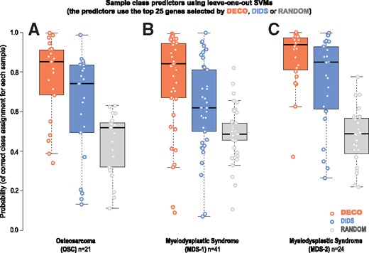
Construction of sample class predictors using a leave-one-out SVM applied to the top DE genes selected by DECO (orange boxplots), by DIDS (blue boxplots) or RANDOM (grey boxplots). Each predictor is built leaving one sample out and using the top 25 genes that are selected by each method with the rest of the samples. In this way n predictors (n=number of samples in each dataset) are constructed. The probability of assigning each sample to its correct class is plotted on the Y-axis. (A): results obtained with the OSC; (B): first MDS-1 and (C): second MDS-2

3.4 Finding hidden variables on a large cancer dataset

To prove that DECO not only outperforms with simulated data or with relatively small datasets, we also tested the method using two large experimental datasets (Table 2). The approach in these tests was changed from group-versus-group comparisons to unsupervised analysis, which did not assume a priori classes or categories. The first dataset selected was a breast cancer (BCC) collection of 285 samples of newly diagnosed tumours divided in oestrogen receptor positive and negative (ESR1+/ESR1–), analyzed for global gene expression profiling with genome-wide RNA microarrays (GEO ID: GSE25055). For this dataset, the unsupervised analysis was carried out using the following input parameters: RDA r = 5, combinations =200 000, adjusted P-value <0.01; NSCA variability explained =97%, feature threshold =3 DEs in at least five samples. The method identified 255 genes with significant differential expression changes (Fig. 6A). The output statistical parameters provided by DECO for these 255 genes are included in Supplementary Material S2. The complete data matrix corresponding to the h-statistic per gene and sample (H, h-statistic matrix) is also provided as Supplementary Material S3.

Fig. 6.

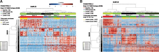
Results of running DECO method to analyze two independent BCC large datasets using unsupervised clustering of patients (samples) and genes (features). Both heatmaps were plotted using the h-statistic values (calculating the distance matrices using 1-Pearson correlation of the h values). (A): heatmap of the h-statistic of 285 patients and 255 DEgs (the expression data for this cohort were obtained with microarrays, from Hatzis et al., 2011); (B): heatmap of the h-statistic of 596 patients and 3228 DEgs (the expression data for this cohort were obtained with RNA-seq, from Ciriello et al., 2015). The samples dendrogram identifies 6 and 5 main subclasses (marked in (A) and (B), respectively). The four standard well-known BCC subtypes (usually associated to the PAM50 signature) (Parker et al., 2009) are labelled with a colour panel close to each heatmap, indicating in brackets the number of samples of each subtype. The newly discovered subclasses identified by the method are marked in yellow. In each heatmap a black box is included to remark a subset of genes associated to the discovered subclasses

DECO found six major subclasses or categories, and indicated that there was a high association between the sample source and a significant subset of genes which marked two subclasses: 2 and 3 in Figure 6A. The samples from primary BCC tumours used for this study were obtained by two different groups: the M. D. Anderson Cancer Center (MDACC, Houston) and the group Investigation of Serial Studies to Predict Your Therapeutic Response (I-SPY) (Hatzis et al., 2011). Each of these two research units used a different procedure to isolate the tumour biopsy samples: (i) 227 samples were obtained by fine-needle aspiration (M. D. Anderson Cancer Center), 210 included in our study; and (ii) 83 samples were obtained by surgical resection of the core biopsy (Investigation of Serial Studies to Predict Your Therapeutic Response), 75 included in our study (Hatzis et al., 2011). We observed in our results how a small group of genes marked a clear difference between these two groups of samples isolated in a different way. This signal was not due to a random selection or to a bad normalization of the data, since more that 95% of the genes did not show any significant difference within these two subclasses. We concluded that those genes were indicating a small change in the expression signal due to differences in the isolation protocols used. In fact, according to the h-statistic provided by DECO, two of the most discriminating genes found for these subclasses were haemoglobin β-subunit and δ-subunit, which have been recently reported to be affected by the procedure of biopsy sampling used in patients with BCC (Tanamai et al., 2009). Together with the signal coming from haemoglobin depletion, the same group of samples showed a strong up-regulation of collagens (COL1A1, COL1A2, COL3A1, COL4A1, COL4A2, COL5A1, COL5A2 and COL6A3), revealing changes in the extracellular matrix components. This dysregulation may be related to different mechanical manipulation of tissue samples, and therefore, related to the isolation procedure. This effect was not reported in the original publication (Hatzis et al., 2011), probably because it affects a small number of genes and does not affect to any critical BCC associated gene. However, we discovered a clear gene change associated to a specific sample phenotype, supporting the value of the DECO algorithm to find confounding or hidden factors. Since these profiles are strongly associated with the sample source, the comparison between two different BCC subtypes (i.e. basal and luminal samples) from different biopsy procedures may have led to the wrong association of these profiles (haemoglobin β-subunit and δ-subunit) with these subtypes of samples. Finally, it is also important to indicate that doing a standard clustering analysis and a derived heatmap based on the gene expression signal did not reveal these gene changes.

Regarding the standard well-known subtypes of BCC, the results of our analysis showed that the h-statistic provided by DECO found the expected division of samples according to the PAM50 subclasses (Parker et al., 2009) (Fig. 6A). Thus, the method was able to find not only the large differences between basal and luminal-like BCC subtypes, but also gene subsets directly related to other subtypes of BCC, more difficult to separate, i.e.: luminal A and luminal B (Fig. 6A).

The method found specific genes associated to basal or luminal PAM50 subtypes (like: GATA3, TBC1D9, EN1, CA12, NAT1, PROM1 and AGR2) that have been previously linked to the ESR1 status in BCC (Wirapati et al., 2008). In fact, a functional enrichment analysis on the genes associated to the basal subtype showed a very significant enrichment in basal up-regulated or down-regulated signatures from MSigDB database in comparison with luminal samples (as defined in the Molecular Signatures Database at the Broad Institute, MSigDB, http://software.broadinstitute.org/gsea/msigdb/).

3.5 Finding disease subtypes using a non-supervised approach on RNA-seq data

DECO was also applied to another large BCC dataset taken from the Cancer Genome Atlas (TCGA) (Cancer Genome Atlas Network, 2012), which includes genome-wide expression profiling using high-throughput RNA-seq. In a recent study, Ciriello et al. (2015) analyzed this dataset discovering a distinct disease inside the BCC tumours corresponding to ‘invasive lobular’ (IL-BCC) subtype, that was clinically and molecularly different to the more common and frequent ‘invasive ductal’ (ID-BCC) subtype. This tumour stratification was not previously investigated because the normal molecular portraits of human breast tumours, even for the datasets of TCGA (Cancer Genome Atlas Network, 2012), followed the most standard classification of BCC in 4 subtypes: luminal A, luminal B, HER2-enriched and basal-like (that is also the one defined by the PAM50 subclasses) (Parker et al., 2009). Under this scenario, we took 596 BCC samples studied by Ciriello et al. (2015) having cases from each one of the 4 main BCC subtypes (n = 307 luminal A, 128 luminal B, 53 HER2-enriched and 108 basal-like), but also including information of the tumour cell type subtypes: IL-BCC and ID-BCC. We analysed this dataset with DECO following an unsupervised procedure, to test if our method was able to find genes as features that distinguished and separated all the different disease subtypes introduced before. For this analysis, we used the original expression RPKM data matrix provided by TCGA, checking a correct normalization and filtering-out 902 genes because they showed low expression in all samples (expression signal RPKM < 2). Consequently, an unsupervised design without any pre-defined category of samples was carried out, setting up the initial DECO parameters to: RDA r = 5; combinations =1 000 000; adjusted P-value <0.01; NSCA variability explained =80%, feature threshold =3 DEs in at least 30 samples.

The results are presented in Figure 6B, and also provided as in Supplementary Material. The heatmap shows the binary clustering of samples and genes obtained using the h-statistic for each sample and gene (Fig. 6B). The method selected 3228 genes that had differential expression changes (according to the threshold indicated above). The values of all the statistical parameters provided by DECO for these 3228 genes are included in Supplementary Material S4. The complete data matrix corresponding to the h-statistic per gene and sample is also provided as Supplementary Material S5. The results showed that the method found four subclasses directly related to the four BCC PAM50 subtypes: subclass 1 corresponding to basal-like subtype (red in Fig. 6B); subclass 2 corresponding mainly to HER2-enriched subtype (blue); subclass 3 to Luminal B subtype (purple) and subclasses 4 and 5 corresponding mainly to Luminal A subtype (marked in green). The method was also able to distinguish a subtype inside Luminal A, assigned to subclass 5 and showing a distinct gene profile. This subtype corresponded to the ‘invasive lobular’ breast cancer (IL-BCC) (marked in yellow in the grey bar in Fig. 6B). Ciriello et al. published a comprehensive molecular portrait of the IL-BCC. Several genes found to differentiate ‘lobular’ from ‘ductal’ breast carcinomas (thrombospondin 4, THBS4, thrombospondin receptor, CD36, multiple cadherins, CDH5, CDH11, CDH17, CDH22, CDH23) (Korkola et al., 2003), were found inside the gene signature that marked subclass 5 according to DECO. By contrast, some genes that showed significant mutations in IL-BCC, like FOXA1 and TBX3 (Ciriello et al. (2015)), but are usually up-regulated in Luminal A samples, were not selected as specific markers of the IL-BCC subtype. Finally, it is important to know that previous studies on BCC indicated that unsupervised clustering of lobular and ductal breast tumours based on expression profiling failed to distinguish between these two subtypes of carcinomas (Korkola et al., 2003).

4 Conclusions

Currently the biomedical scientific community is trying to resolve the problem of samples heterogeneity through different and varied proposals: remove unwanted variation, better outlier detection, robust machine learning, single-cell analyses, etc. This problem is very relevant in cancer studies due to highly intra- and inter-tumour heterogeneity (Gyanchandani et al., 2016; Rubio-Perez et al., 2015). Interestingly, COPA method, after more than a decade from its publication, is still used to find outlier profiles due to its simplicity (Gaykalova et al., 2017; Teng et al., 2016; Wu et al., 2017), despite the fact that it is not the best method.

The new method proposed here, DECO, has been designed to analyze the variability in complex omic-scale datasets including multiple sample subtypes and heterogeneous changes in specific features. Under this framework, our method aims to detect any relevant feature supporting the intrinsic heterogeneity through a subsampling procedure without replacement (RDA). The feature selection process is crucial for any posterior analysis (Singh and Sivabalakrishnan, 2015) because it allows us not only select and rank significant features but also place in context which samples are aiding this variability. Thus, the Standard Chi-Square score (S_f) was implemented to facilitate the ranking of features found instead a simple counter of DEs (or repeats). Noteworthy, subsampling and other resampling techniques have been broadly used in many scientific fields for statistic estimation, stability assessment or learning processes. If they are carefully raised (involving previous knowledge, computational cost or suitability of the problem to solve), these techniques provide useful and reliable information (Gur-Dedeoglu et al., 2008; Irizarry et al., 2003; Lee et al., 2014). Although big data analyses are coming more frequent now, summarizing it into smart data remains essential and requires of the development of new exhaustive approaches.

Our method DECO, and particularly the RDA step, adds a new scheme analysis on a very acknowledged differential analysis approach like LIMMA and its Bayesian (eBayes) method (Smyth, 2004), enlarging the suitable profiles from complete changes to all our four model-types and ranking them accordingly. However, it is important to mention that LIMMA is partially based on t-test statistics, then the sample size of compared samples (subsampling size per iteration) roughly affects to its statistical power (Dobbin and Simon, 2005; Stretch et al., 2013). We consider that approaching the feature selection or differential analysis through a subsampling scheme, as provided by RDA, release to gain insight into the significant variability present at any homo- or heterogeneous omic dataset.

We have shown that DECO improves well-established statistical methods that analyze differential signal for the detection of outlier features, and outperforms other procedures on the capability to identify relevant subclasses within a cohort of samples. Thus, the method is applicable both to find subtle differences among pre-defined classes or subclasses of samples that present a differential behaviour marked by specific features. The search for molecular features that define specific individuals is a key objective of personalized medicine.

All the examples run in this publication were focussed on genome-wide expression datasets. These types of data were selected because they study complex disease scenarios on well-characterized patient clinical cohorts. Currently, one of the most common scopes in genomic profiling and genome-wide data analyses is to find better biomarkers for specific pathological states that can define new diseases and disease subtypes. However, since LIMMA has been broadly applied to several different omic platforms (i.e. proteomic, miRNA and DNA methylation data) and it is the functional core of RDA step, DECO is greatly suitable to be applied on these platforms. In fact, there are many publications in the last decade reporting its use for proteomics differential analysis due to its simplicity, performance and dealing with variability of proteomic data (Basken et al., 2018; Jeannin et al., 2018; Kuzniar et al., 2017; Margolin et al., 2009; Pagel et al., 2015; Ting et al., 2009), for miRNA differential analysis (Mastriani et al., 2018; Thomou et al., 2017; Xue et al., 2017), and there are also many successful publications where LIMMA have been applied for differential analysis of CpG methylation levels in different biological scenarios (Johnson et al., 2017; Martorell-Marugan et al., 2019; Saito et al., 2017; Stefan et al., 2014; Wockner et al., 2014). For all these reasons, we think the workflow followed by DECO can be of great help for better disease stratification and biomarker identification.

Acknowledgements

We acknowledge the funding provided to JDLR research group by the Spanish Ministry of Economy, Industry and Competitiveness (MINECO) with grants of the ISCiii co-funded by FEDER (references AC14/00024 and PI15/00328); as well as funding provided to JDLR by the European Commission, EU Horizon 2020 Programme project ArrestAD (reference H2020-FETOPEN-1-2016-2017, Project ID: 737390). We also acknowledge the provision of research funding by Celgene Research SLU (Celgene Institute for Translational Research Europe, CITRE), a wholly owned subsidiary of Celgene Corporation, to enable collaborative work among researchers at CiC-IBMCC (CSIC/USAL) and CITRE researchers.

Funding

This work was supported by the research grant [AC14/00024], from the Instituto de Salud Carlos III (ISCiii) co-funded by the Fondo Europeo de Desarrollo Regional (FEDER). A PhD research grant to F.J.C.L. (from the Programme Ayudas a la Contratación de Personal Investigador) provided by the Junta de Castilla y Leon (JCyL) with the support of the Fondo Social Europeo (FSE) is also acknowledged. C.F. received funding from the Spanish Ministry MINECO, Torres-Quevedo Programme [reference PTQ-13-06319].

Conflict of Interest: none declared.