


Abstract
Recent technology developments have made it possible to generate various kinds of omics data, which provides opportunities to better solve problems such as disease subtyping or disease mapping using more comprehensive omics data jointly. Among many developed data-integration methods, the similarity network fusion (SNF) method has shown a great potential to identify new disease subtypes through separating similar subjects using multi-omics data. SNF effectively fuses similarity networks with pairwise patient similarity measures from different types of omics data into one fused network using both shared and complementary information across multiple types of omics data.
In this article, we proposed an association-signal-annotation boosted similarity network fusion (ab-SNF) method, adding feature-level association signal annotations as weights aiming to up-weight signal features and down-weight noise features when constructing subject similarity networks to boost the performance in disease subtyping. In various simulation studies, the proposed ab-SNF outperforms the original SNF approach without weights. Most importantly, the improvement in the subtyping performance due to association-signal-annotation weights is amplified in the integration process. Applications to somatic mutation data, DNA methylation data and gene expression data of three cancer types from The Cancer Genome Atlas project suggest that the proposed ab-SNF method consistently identifies new subtypes in each cancer that more accurately predict patient survival and are more biologically meaningful.
The R package abSNF is freely available for downloading from https://github.com/pfruan/abSNF.
Supplementary data are available at Bioinformatics online.
1 Introduction
With the recent development of high-throughput technology, a vast amount of omics data such as mutations, copy number variants, DNA methylation data and gene expression data have been generated, which help advance understanding in system biology. A review paper on integrative genomics in cancer emphasizes a fundamental principle which says ‘any biological mechanism builds on multiple molecular phenomena, and only through the understanding of the interplay within and between different layers of genomic structures can one attempt to fully understand phenotypic traits’ (Kristensen et al., 2014). The development of powerful integrative analysis tools for multi-omics data to better understand biological processes is a natural next step. Many studies have indicated associations between cancer subtypes and tumor aggressiveness, prognoses and responses to therapy, which suggests clinical potential with cancer type distinctions (Hu et al., 2006; Neve et al., 2006; Rouzier et al., 2005; Sørlie et al., 2001). Several successful examples that translate cancer genomic discoveries into therapeutics and diagnostics exist and reinforce the importance of cancer omics in personalized cancer medicine (Chin et al., 2011).
Many integrative methods for clustering have been developed lately. One common initial strategy in disease subtyping with multi-omics data is to first cluster samples using one type of omics data and then further cluster group labels from each type of omics data. This is usually referred to as the consensus clustering method (Cancer Genome Atlas Network, 2012; Cancer Genome Atlas Research Network, 2016; Monti et al., 2003). Lock et al. (2013) proposed a method which decomposes variation of an integrated multi-source dataset into three terms: a joint variation across sources, a structured variation individual to each source and residual noise. Qin (2008) and Lee et al. (2008) proposed clustering methods on correlation matrices between any two types of omics data. This line of methods utilizes shared information across multi-omics data in order to identify their common patterns. To capture both common and complementary information across multi-omics data, a latent variable model, iCluster, was developed (Shen et al., 2009). A major extension of the original algorithm, iClusterPlus, that allows a joint modeling of discrete and continuous data types and a substantially faster implementation was also developed (Mo et al., 2013). A more recent extension of iCluster uses a full Bayesian latent variable approach (Mo et al., 2018) and allows further improvement in terms of statistical inference on feature selection. Another multiple dataset integration (Kirk et al., 2012) method similarly implements a Bayesian latent variable model. Both iCluster, multiple dataset integration and most of other clustering methods have a pre-selection step to screen features, making them sensitive to features pre-selected. Recently, Wang et al. (2014) developed a similarity-based method that generates similarity measures between pairwise subjects using one type of omics data first, referred to as the patient similarity network, and then iteratively updates individual similarity networks from individual types of omics data using information from other types of omics data. Similarity networks from multiple types of omics data are thus fused and the method is referred to as similarity network fusion (SNF). Other similar method such as the affinity network fusion (Ma and Zhang, 2018) was also developed lately. Like any similarity-based methods, no pre-screening feature selection step is necessary, which avoids the potential to screen out any signal features especially ones with weak signals. However, it is also acknowledged that in similarity-based methods, unscreened noise features may dilute clustering signals and weaken the study power. To alleviate this disadvantage, different omics features may be weighted differently in the construction of the similarity measures to up-weight signal features and down-weight noise features. This idea has been adopted in similarity-based methods in genome-wide association studies (Wessel and Schork, 2006). With multi-omics data, Xu et al. (2016) proposed a weighted SNF method that utilizes miRNA-TF-mRNA regulatory network in identifying cancer subtypes. However, this method is limited to the specific types of omics data and the databases used to construct the regulatory network do not cover all true interactions either.
In this paper, we proposed a more general framework of weighted SNF method: an association-signal-annotation boosted SNF (ab-SNF) method that incorporates association signal annotations between features of different omics data and outcome of interest as weights in the construction of similarity measures between any given pair of samples in order to boost the clustering performance. Specifically, in the proposed ab-SNF method, for each type of omics data, we first construct feature-level weights using association signal annotations between individual features and outcomes, and then compute the corresponding association-signal-annotation boosted similarity matrices. These similarity matrices can be considered as similarity networks of samples whose nodes are subjects and edges are pairwise similarity measures between any given pair of samples. We then fuse the boosted similarity networks from individual types of omics data into a single boosted similarity network through a non-linear combination method. This non-linear combination method iteratively updates the boosted similarity networks from individual types of omics data using the boosted similarity networks of other types (Blum and Mitchell, 1998; Wang et al., 2012) and amplifies the effects of the feature-level association-signal-annotation weights.
We conducted simulation studies to compare the performances of the proposed ab-SNF method and methods that either are not boosted or do not integrate multi-omics data and observed a much improved performance of the ab-SNF method in identifying true disease subtypes. Most importantly, we observed that the improvement in the clustering performance is due to the amplified effects of feature-level weights across multiple types of omics data through iterations of the diffusion process that integrates multi-omics data. We applied the ab-SNF method to somatic mutation, DNA methylation and gene expression data of breast invasive carcinoma (BRCA), kidney renal papillary cell carcinoma (KIRP) and liver hepatocellular carcinoma (LIHC) from The Cancer Genome Atlas (TCGA) project and subtyped cancer patients that more accurately reflect their survival than those by the original SNF method without association-signal-annotation weights across the three independent cancer types consistently.
2 Materials and methods
All continuous features of different types were first normalized to have mean zero and unit standard deviation. For discrete features such as somatic mutations, we worked on gene-level and considered a gene to be mutated if there is any mutation on that gene and coded the gene to be ‘1’ and ‘0’ otherwise.
There are three steps in the proposed ab-SNF method: (i) constructing feature-level weights and association-signal-annotation boosted similarity networks for individual types of omics data; (ii) fusing multiple boosted similarity networks into one single integrated boosted similarity network and (iii) subtyping disease subjects based on the integrated boosted similarity network (Fig. 1).
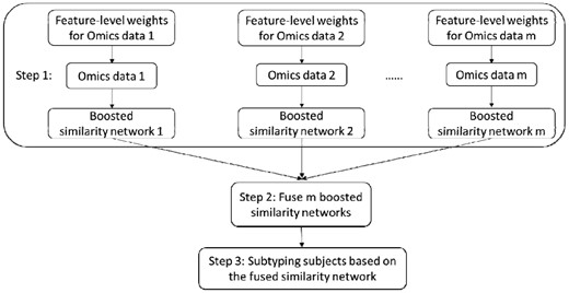
The pipeline of the proposed ab-SNF method
2.1 Constructing boosted similarity networks for individual types of omics data
2.1.1 Feature-level weights
For individual types of omics data, we consider features that can better differentiate tumor samples from adjacent normal samples (or independent normal samples) as potential signal features for subtyping tumor samples, i.e. features with stronger association signals with outcomes of interests. We would want to up-weight these signal features in constructing the patient similarity network using this type of omics data. Therefore, for a continuous feature k such as an epigenetic feature (DNA methylation at a CpG site) or a transcriptomic feature (gene expression of a gene), we weight the feature using the feature-level association P-value pk from comparing tumor samples to adjacent normal samples (or independent normal samples) at feature k, using such as the paired t-test (or the two-sample t-test). The feature-level weight wk for feature k is then defined as , where K is the total number of features of that type. For a binary feature k, such as a mutation gene, we can select mutation genes that are known to be cancer-related based on the Cancer Gene Census (CGC) (Futreal et al., 2004) database. This is equivalent to set feature-level weight wk = 1 for mutation gene k in the CGC database and wk = 0 for all other mutation genes.
2.1.2 Association-signal-annotation boosted patient similarity networks
Here is the average distance between tumor sample i and his/her neighbors , where are tumor samples with the smallest distances to tumor sample i (Yang et al., 2008) and is set at 20 as the default (Wang et al., 2014). These weighted similarity measures between any given pairs of tumor samples i and j, comprises the boosted patient similarity network .
2.2 Fusing multiple boosted similarity networks
The network fusion algorithm was originally developed in the area of computer vision (Blum and Mitchell, 1998; Wang et al., 2012). For the mth type of omics data, we first define a global boosted similarity network and a local boosted similarity network using the boosted similarity network defined in Equation (2.1). Specifically, the entries of the global boosted similarity network are defined as the normalized entries in between any pairs of tumor samples. The entries of the local boosted similarity network are defined as the normalized entries in between tumor sample i and his/her neighbors , where was defined in Section 2.1.2, and 0 between tumor sample i and tumor samples outside of his/her neighbors . This local boosted similarity network is constructed with an assumption that local similarities might be more reliable than remote ones.
There are three important observations of the diffusion process: (i) if subjects i and j are similar in all types of omics data, the diffusion process will make them even closer; (ii) if subjects i and j are not similar in one type of omics data but similar in other types, the similarity that exists in one type of omics data will be propagated through the diffusion process and (iii) the effects of feature-level association-signal-annotation weights are amplified across multiple types of omics data through iterations of the diffusion process.
2.3 Subtyping subjects based on the integrated boosted similarity network
We apply the spectral clustering method on the fused boosted similarity network which utilizes eigenvectors of the graph Laplacian of the similarity network to accomplish subject clustering (Ng et al., 2002). To determine the number of clusters, i.e. disease subtypes, we used the eigengap method (Ng et al., 2002). Specifically, we sorted the eigenvalues of the Laplacian matrix in an ascending order. The eigengaps are defined as the differences between consecutive eigenvalues. The best number of clusters, C, is the number that maximizes the Cth eigengap. For well-studied cancer types such as BRCA, when at least five breast cancer subtypes are already widely accepted (Parker et al., 2009), we will examine the number of clusters starting from 6. Finally, we remove clusters with fewer than 10 subjects to ensure stable results.
3 Simulation studies
3.1 Comparison methods
We conducted simulation studies to investigate the performance of the ab-SNF method and compared to that of (i) the original SNF without weights, (ii) methods that use only one type of omics data with/without weights and (iii) methods that use two types of omics data with/without weights. These simulation studies can help demonstrate how feature-level weights improve disease subtyping and how the effects of feature-level weights can be amplified when integrating multi-omics data.
3.2 Simulation settings
In each simulation setting, we considered 200 tumor samples with three types of omics data. We set the 200 tumor samples from four subtypes A, B, C and D each with 50 tumor samples. There are 1000 features in each type with 5% informative in defining subtypes. The simulation studies were designed such that using one type data, we can only separate two of the four subtypes from the other two. Only when we use information from all three types, can we separate all four subtypes. Specifically, for one type of data such as gene expression data, we generated expression levels of the 50 signal features from a normal distribution N(−1, 2) for samples of subtypes A and B to represent down-regulated gene expression and from a normal distribution N(1, 2) for samples of subtypes C and D. For the second type of data such as DNA methylation data, we generated methylation levels of the 50 signal features from a normal distribution N(−1, 2) for samples of subtypes A and C to represent hypo-methylation and from a normal distribution N(1, 2) for samples of subtypes B and D. Measures of each of the 950 noise features for these two types of data were generated from a normal distribution N(0, 2). For the third type of data such as somatic mutation data, we generated mutation status (‘1’ for mutation and ‘0’ otherwise) for the 50 signal features from a Bernoulli distribution Bernoulli(0.4) for samples of subtypes A and D and from Bernoulli(0.2) for samples of subtypes B and C. Measures of the 950 noise features for mutation data were generated from a Bernoulli distribution Bernoulli(0.1). We simulated 1000 datasets for each simulation setting.
We considered simulation scenarios to investigate how feature-level weights affect the clustering performance (Table 1). Specifically, we examined how (i) percent and magnitude of correctly up-weighted or incorrectly down-weighted signal features out of all true signal features and how (ii) percent and magnitude of correctly down-weighted or incorrectly up-weight noise features out of all true noise features affect the performance of the ab-SNF method in disease subtyping. As defined in Section 2.1.1, feature-level weights are based on association-signal-annotation P-values: , which are values in between 0 and 1. We estimated feature-level weights using TCGA data where ranges of weights for potential signals and noises were obtained. We then rescaled the estimated weights for easier illustration, based on which we simulated different feature-level weights, either up-weighted or down-weighted, from uniform distributions. Specifically, we generated up-weights for signals from Uniform(1, 2), Uniform(1, 3) or Uniform(1, 4). We also generated down-weights from Uniform(0, 1), Uniform(0.7, 1), Uniform(0.3, 0.7) or Uniform(0, 0.3). We also set different percent of correctly up-weighted signal features and different percent of correctly down-weighted noise features.
Simulation scenarios and corresponding results
| Simulation scenarios | Signal features | Noise features | Accuracy%a of each method | ||||||||
|---|---|---|---|---|---|---|---|---|---|---|---|
| Info%b | Magnitude | Uninfo%c | Magnitude | Med alone | Gee alone | Muf alone | Me+ Ge | Me+ Mu | Ge+ Mu | Me+Ge+ Mu | |
| Not boosted scenario | 100 | 1 | 100 | 1 | 47.34 | 47.34 | 42.92 | 62.80 | 52.66 | 52.66 | 69.29 |
| Boosted scenario I | 20 | U(1, 3) | 40 | U(0, 1) | 47.69 | 47.69 | 42.94 | 69.04 | 57.33 | 57.33 | 83.24 |
| 60 | U(1, 3) | 40 | U(0, 1) | 47.82 | 47.82 | 42.97 | 71.17 | 59.79 | 59.79 | 88.45 | |
| 100 | U(1, 3) | 40 | U(0, 1) | 48.47 | 48.46 | 43.04 | 73.45 | 61.50 | 61.50 | 91.44 | |
| Boosted scenario II | 60 | U(1, 2) | 40 | U(0, 1) | 47.44 | 47.44 | 42.95 | 69.69 | 58.02 | 58.02 | 84.32 |
| 60 | U(1, 3) | 40 | U(0, 1) | 47.82 | 47.82 | 42.97 | 71.17 | 59.79 | 59.79 | 88.45 | |
| 60 | U(1, 4) | 40 | U(0, 1) | 47.99 | 47.99 | 43.49 | 72.00 | 61.53 | 61.53 | 90.94 | |
| Boosted scenario III | 60 | U(1, 3) | 0 | U(0, 1) | 47.46 | 47.46 | 42.98 | 70.25 | 58.65 | 58.64 | 85.09 |
| 60 | U(1, 3) | 40 | U(0, 1) | 47.82 | 47.82 | 42.97 | 71.17 | 59.79 | 59.79 | 88.45 | |
| 60 | U(1, 3) | 80 | U(0, 1) | 48.47 | 48.47 | 43.44 | 73.19 | 62.05 | 62.05 | 92.30 | |
| Boosted scenario IV | 60 | U(1, 3) | 40 | U(0.7, 1) | 47.87 | 47.87 | 42.96 | 70.18 | 59.08 | 59.08 | 86.67 |
| 60 | U(1, 3) | 40 | U(0.3, 0.7) | 47.98 | 47.98 | 43.16 | 71.88 | 60.15 | 60.15 | 88.01 | |
| 60 | U(1, 3) | 40 | U(0, 0.3) | 48.13 | 48.14 | 43.50 | 71.97 | 61.42 | 61.42 | 89.64 | |
| Boosted scenario V | 60 | U(0, 1) | 40 | U(0, 1) | 46.36 | 46.36 | 42.09 | 56.21 | 48.79 | 48.79 | 57.11 |
| 60 | U(1, 3) | 40 | U(1, 3) | 47.17 | 47.17 | 42.4 | 62.51 | 53.57 | 53.57 | 71.69 | |
| 60 | U(0, 1) | 40 | U(1, 3) | 42.14 | 42.13 | 40.97 | 38.14 | 37.93 | 37.93 | 37.44 | |
aAccuracy% stands for percent of subjects being correctly clustered.
bInfo% stands for percent of true signal features (informative features) being correctly up-weighted.
cUninfo% stands for percentage of true noise features (uninformative features) being correctly down-weighted.
dMe stands for DNA methylation.
eGe stands for gene expression.
fMu stands for mutation.
We also conducted additional simulation studies to investigate how the proposed ab-SNF method performs if certain types of omics data are pure noise and not help define subtypes. The detailed description of the addition simulation settings is included in the Supplementary Materials.
3.3 Simulation results
We examined how accurately each method identifies true disease subtypes, where we define the accuracy as the percent of subjects being correctly clustered. Table 1 summarizes simulation results. It is clear that the methods with association-signal-annotation weights achieved higher accuracies than their corresponding no-weight versions. The ab-SNF method using all three types of data achieved the highest accuracies in scenarios I–IV, where different percentages of true signal features were correctly up-weighted with different magnitudes, and different percentages of noise features were correctly down-weighted with different magnitudes. Specifically, in scenario I, when the magnitude of weights for signal features were from Uniform(1, 3), i.e. signal features being correctly up-weighted, and the magnitude of weights for noise features were from Uniform(0, 1), i.e. noise features being correctly down-weighted, and 40% noise features were down-weighted while increasing the percentage of up-weighted signal features, the clustering accuracy of the ab-SNF method was the highest as expected. For the comparison methods that use only one type of data, up-weighting signal features and down-weighting noise features only slightly improves the clustering accuracy. For the comparison methods that use two types of data, the improvements in clustering accuracies by up-weighting signal features and down-weighting noise features were larger than those of methods using only one type of omics data. Moreover, for the comparison methods that use all three types of data, up-weighting signal features and down-weighting noise features achieved the largest improvements in clustering accuracies. This indicates that the effects of feature-level weights can be amplified when multi-omics data are integrated. The original SNF methods that integrate information from two or three types of data without feature-level weights has an improved clustering accuracy than that of the methods that only use one type of omics data with/without weights. These suggest that (i) integrating multiple types of omics data accumulates more information thus improves the clustering accuracy as previously already demonstrated; and (ii) the improvement from correctly up-weighting signal features and down-weighting noise features in multiple types of omics data could be amplified during the integration of these multiple types of omics data through the diffusion process [Equations (2.3) and (2.4)].
Similar patterns can be observed in scenarios II–IV, where the clustering accuracy of the ab-SNF method increases as the magnitude of weights for signal features increases, as the percentage of noise features being correctly down-weighted increases, and as the magnitude of weights for noise features decreases, respectively.
In scenario V, the clustering accuracy of the ab-SNF method increases much slower as the magnitude of weights of correctly up-weighted signal features increases but the magnitude of weights of incorrectly up-weighted noise features also increases. As an extreme setting in scenario V, which would rarely happen in real data, when 60% of signal features were incorrectly down-weighted and 40% of noise features were incorrectly up-weighted, the clustering accuracy of the ab-SNF method is lower than that of the original SNF method. This emphasizes that the feature-level weights could be very useful but it is important to assign correct weights to individual features.
In the additional simulation studies investigating how the proposed ab-SNF method performs if certain types of omics data are pure noise and not help define subtypes, we observed similar patterns in the results. That is, integrating a data type that is pure noise decrease the clustering accuracy as expected. However, feature-level weights help minimize the drop in accuracy. The detailed simulation results for the additional simulation settings are included in the Supplementary Materials.
4 Real data applications
4.1 TCGA cancer data
To demonstrate the performance of the proposed ab-SNF method in cancer subtyping, we worked on three independent cancer types from TCGA, i.e. BRCA, KIRP and LIHC, each with three types of omics data., i.e. somatic mutation data, DNA methylation 450 K array data, and gene-level RNA-seq data. This is based on the biological assumption that cancer-related mutations may change genome-wide methylation levels, which then may lead to changes in gene expression (Jones, 2012).
We conducted the same quality control steps across the three cancer types where we removed tumor samples with more than 30% missing in any of the three data types. We then removed features with more than 30% missing. After these two steps, for the rest of the missingness in gene expression and DNA methylation data, we imputed using K-nearest neighbor (Troyanskaya et al., 2001). We also conducted batch effect correction for gene expression using Combat (Johnson et al., 2007). For DNA methylation, we further removed CpG sites on sex chromosomes and CpG sites overlapping with known single nucleotide polymorphisms and also corrected type I/II probe bias using wateRmelon (Pidsley et al., 2013). To generate feature-level association signal annotations, we used additional data including gene expression measures of adjacent normal samples next to tumor samples, and DNA methylation 450 K measures of adjacent normal samples next to tumor samples. Detailed descriptions of the TCGA BRCA, KIRP and LIHC datasets are provided in the Supplementary Materials.
Existing researches have integrated multiple omics data such as copy number variants and gene expression for breast cancer subtyping (Curtis et al., 2012), copy number variants, gene expression, DNA methylation, microRNA expression and protein expression for renal cancer subtyping (Cancer Genome Atlas Research Network, 2016) and copy number variants, DNA methylation, gene expression, microRNA expression and proteomics data for liver cancer subtyping (Ally et al., 2017). We will compare subtyping results using the ab-SNF method to published results for each individual cancer type.
4.2 Overall performance of the ab-SNF method in three independent cancer types
For each cancer type, we applied the spectral clustering method on the integrated boosted similarity network generated by the ab-SNF method as well as similarity networks generated by the comparison methods. For each cancer type, Table 2 displays the number of subtypes constructed by each method based on the eigengap criteria introduced in Step 3 of the algorithm. The subtypes identified by the ab-SNF method are most significantly associated with patient survival across all comparison methods in all three cancer types. Consistent with what we observed in the simulation studies, based on the log-rank P-values that associate subtypes and patient survival in each individual cancer type, the comparison methods that use only one type of omics data with feature-level weights are only slightly better than the non-weight versions. When integrating multi-omics data with weights, the subtypes generated have much stronger association with patient survival than that generated by the original SNF. This suggests that the effects of weights were amplified during the diffusion process when multiple types of omics data were integrated.
Subtype analyses in three TCGA cancer types with (i) best chosen number of clusters based on the eigengap criteria in parentheses, (ii) number of clusters after filtering out clusters whose sizes <10 in bold font and (iii) corresponding survival P-values
| Cancer types | Mua alone | Weighted Mu | Meb alone | Weighted Me | Gec alone | Weighted Ge | SNF | ab-SNF | |
|---|---|---|---|---|---|---|---|---|---|
| BRCA | Number of clusters | 7 (7) | 7 (8) | 6 (7) | 7 (8) | 6 (6) | 7 (7) | 4 (7) | 8 (8) |
| Survival P-values | 0.18 | 0.28 | 0.48 | 0.16 | 0.13 | 0.12 | 0.10 | ||
| KIRP | Number of clusters | 3 (3) | 4 (4) | 3 (3) | 4 (4) | 3 (5) | 4 (4) | 3 (3) | 4 (4) |
| Survival P-values | 0.65 | 0.081 | |||||||
| LIHC | Number of clusters | 3 (3) | 4 (4) | 3 (3) | 4 (4) | 3 (3) | 3 (3) | 3 (3) | 5 (5) |
| Survival P-values | 0.21 | 0.12 | 0.16 | 0.15 | 0.91 | 0.44 | 0.26 | 0.046 |
aMu stands for mutation.
bMe stands for DNA methylation.
cGe stands for gene expression.
We also used C-index to measure the prediction accuracy of each model for each cancer type, where a C-index of 1 indicates perfect prediction and a C-index of 0.5 indicates random guess. C-indexes of the ab-SNF method are 0.69, 0.87 and 0.63 for BRCA, KIRP and LIHC, respectively, while the corresponding C-indexes using the original SNF method are 0.61, 0.83 and 0.55.
4.3 Individual cancer case studies
4.3.1 TCGA BRCA
BRCA subtyping has been extensively studied. Parker et al. (2009) identified a classifier with 50 genes and defined 5 BRCA subtypes using gene expression of these 50 genes, which has been widely applied and referred as PAM 50. Curtis et al. (2012) identified 10 BRCA subtypes using copy number variants and gene expression data.
Here using mutation data, DNA methylation data and gene expression data, the ab-SNF method identified eight BRCA subtypes. These eight subtypes are associated with survival with a P-value of (Table 2) while the original SNF method identified seven subtypes which are associated with survival with a P-value of 0.057. However, 3 subtypes out of the 7 have fewer than 10 subjects and were thus removed. The rest four subtypes are associated with survival with a P-value of 0.10 (Table 2).
Figure 2a plots the Kaplan–Meier curves of the eight BRCA subtypes constructed by the ab-SNF method. We note that the smallest subtype with 14 subjects has the worst survival with a mean survival time of 1128 days. This subtype also has the highest averaged mutation burden (Fig. 2d). Among the 4 subtypes identified by the original SNF method, these 14 subjects were clustered into two different subtypes with a mean survival time of 2763 and 2650 days, respectively, i.e. the 14 subjects survived much shorter than other subjects in these two subtypes. This suggests that the ab-SNF method might be able to subtype BRCA patients more accurately reflect their survival.
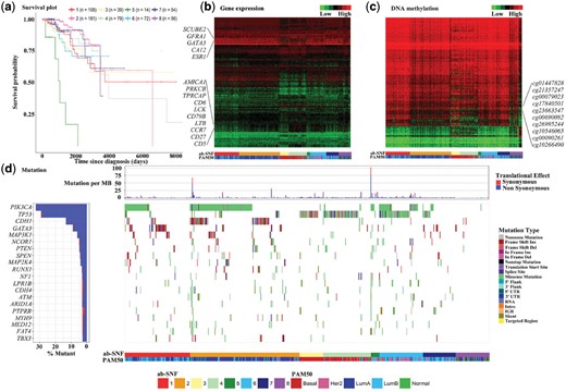
(a) Kaplan–Meier curves of the eight TCGA BRCA subtypes identified by the ab-SNF method with the number of subjects in each subtypes. (b) Heatmap of gene expression profiles of the top ranked 500 genes by feature-level weights across the eight BRCA subtypes identified by the ab-SNF method compared with the PAM50 subtypes. (c) Heatmap of DNA methylation profiles of the top ranked 500 CpGs by feature-level weights across the eight BRCA subtypes identified by the ab-SNF method compared with the PAM50 subtypes. (d) The left panel displays the mutation frequencies of the top ranked 20 mutation genes by mutation frequencies across all BRCA subjects. The top chart in the right panel displays the mutation burdens, defined as the number of mutations per million basepair, across the eight BRCA subtypes. The bottom chart in the right panel displays the mutation profiles of these 20 mutation genes by mutation types across the eight BRCA subtypes
Figure 2b displays the heatmap of gene expression levels of the top ranked 500 genes by feature-level association weights for the eight BRCA subtypes by the ab-SNF method. We clearly see different gene expression patterns across the eight subtypes. For example, comparing subtypes 1 and 2, subtype 1 has lower gene expression levels for several CGC genes such as CD79B and LCK. Subtype 4 has higher gene expression levels than those of subtype 3 at these two genes. Subtypes 3 and 4 have lower gene expression levels than subtypes 1 and 2 at genes such as GATA3, which is an important breast cancer gene (Takaku et al., 2015). Figure 2c similarly displays the heatmap of DNA methylation levels of the top ranked 500 CpGs by feature-level weights. Different patterns of DNA methylations across the eight subtypes can be similarly observed. For example, comparing subtype 2 to subtypes 1, 6 and 7, methylation levels at CpGs such as cg26995244, cg10546065 and cg17840501 are lower in subtype 2, and even lower in subtypes 3, 4 and 8. Note that cg26995244 and cg10546065 are on gene PRR5, and cg17840501 is on gene SEPT9, when PRR5 and SEPT9 are both important breast cancer genes (Connolly et al., 2011; Johnstone et al., 2005). We further investigate the mutation landscape of the top ranked mutation genes by mutation-frequency across subjects in the eight BRCA subtypes (Fig. 2d). The frequencies of mutation genes vary significantly across the eight subtypes. For example, about 40–60% subjects in subtypes 1, 2, 5 and 6 have functional mutations in the PIK3CA gene. In contrast, the PIK3CA functional mutation only occurred in 2–5% of subjects in subtypes 3, 4 and 8 and 11% of subjects in subtype 7. Other important breast cancer genes such as TP53, CDH1, GATA3, MAP3K1, NCOR1 and PTEN also show different mutation patterns across the eight subtypes.
To further investigate the clinical meaning of the eight subtypes, we summarized comprehensive characteristics of the eight subtypes through comparing the genomic, clinical and proteomics features summarized in a review paper on comprehensive molecular portraits of human breast tumors (Cancer Genome Atlas Network, 2012). Specifically, subtypes 3 and 4 are mostly basal-like, as (i) most (75–80%) of the subjects have TP53 mutations (Fig. 2d), (ii) are hypo-methylated (Fig. 2c), (iii) have low estrogen receptor (ER)-positive rates [13 and 25%, respectively, among subjects with ER status available (Table 3)] and (iv) have low HER2-positive rates [0 and 8%, respectively, among subjects with HER2 status available (Table 3)]. Subtype 6 is mostly HER2-enriched, as (i) 71% of the subjects have TP53 mutations and 47% have PIK3CA mutations (Fig. 2d), and (ii) have a relatively high HER2-positive rate [29% among subjects with HER2 status available, note that the average percentage of HER2-postive rate for other 7 subtypes is 9% (Table 3)]. Subtype 2 is mostly Luminal A, as (i) more than half (57%) of the subjects have PIK3CA mutations (Fig. 2d), (ii) have very high ER-positive rate [97% among patients with ER status available (Table 3)] and (iii) have low HER2-positive rate [11% among patients with HER2 status available (Table 3)]. Subtype 7 is mostly Luminal B, as (i) the most frequently mutated genes are PIK3CA (25%) and TP53 (12%) and (ii) have very high ER-positive rate [96% among subjects with ER status available (Table 3)] and (iii) have low HER2-positive rate [18% among patients with HER2 status available (Table 3)]. Subtype 1 is a combination of Luminal A and Luminal B (Fig. 2d).
Clinical characteristics of the subjects in the eight TCGA BRCA subtypes identified by the ab-SNF method
| Subtypes by ab-SNF | ER status | HER2 status | ||||||
|---|---|---|---|---|---|---|---|---|
| Not evaluated | Negative | Positive | Not evaluated | Equivocal | Indeterminate | Negative | Positive | |
| 1 (n = 108) | 6 | 4 | 98 | 28 | 21 | 3 | 48 | 8 |
| 2 (n = 181) | 5 | 5 | 171 | 25 | 31 | 2 | 106 | 17 |
| 3 (n = 39) | 1 | 33 | 5 | 6 | 9 | 0 | 24 | 0 |
| 4 (n = 79) | 4 | 56 | 19 | 18 | 10 | 1 | 45 | 5 |
| 5 (n = 14) | 2 | 3 | 9 | 3 | 1 | 0 | 4 | 6 |
| 6 (n = 72) | 6 | 15 | 51 | 9 | 12 | 1 | 32 | 18 |
| 7 (n = 54) | 6 | 2 | 46 | 10 | 17 | 2 | 17 | 8 |
| 8 (n = 56) | 2 | 12 | 42 | 9 | 10 | 0 | 34 | 3 |
The ab-SNF method also identified several novel subtypes. Subtype 5 has the worst survival (Fig. 2a) and is characterized by a high ER-positive rate [75% among subjects with ER status available (Table 3)] and a high HER2-positive rate [55% among subjects with HER2 status available (Table 3)], when none of the previously identified BRCA subtypes have such characteristics. Subtype 8 is characterized by a low mutation burden (Fig. 2d) and low mutation rates at TP53 (2%) and PIK3CA (0%), a high ER-positive rate [78% among subjects with ER status available (Table 3)] and a low HER2 positive rate [6% among subjects with HER2 status available (Table 3)], when none of the previously identified BRCA subtypes have such characteristics. This indicates that the subtypes identified by the ab-SNF method may provide additional clinical insights for BRCA.
4.3.2 TCGA KIRP and TCGA LIHC
We conducted similar analyses for KIRP and LIHC. KIRP subtyping has also been studied. TCGA network identified four KIRP subtypes using copy number variants, mRNA expression data, DNA methylation data, microRNA expression data and proteomics data (Cancer Genome Atlas Research Network, 2016). Here the ab-SNF method also identified four KIRP subtypes that are associated with survival with a P-value of (Table 2). The original SNF method identified three KIRP subtypes that are associated with survival with a P-value of (Table 2). LIHC subtyping has also been studied. TCGA network identified three LIHC subtypes using copy number variants, mRNA expression data, DNA methylation data, microRNA expression data and proteomics data (Ally et al., 2017). Here the ab-SNF method identified five LIHC subtypes that are associated with survival with a P-value of 0.046 (Table 2). The original SNF method identified three LIHC subtypes that are associated with survival with a P-value of 0.26 (Table 2). The detailed investigation of the subtypes of these two cancer types is included in the Supplementary Materials.
4.4 Empirical analysis of the eigengap criteria to select number of clusters
To investigate the effectiveness of using the eigengap criteria to choose the number of clusters with spectral clustering, we conducted an empirical analysis, where we pooled all 901 tumor samples of BRCA, KIRP and LIHC cancer types together. Here we know the true number of clusters with pooled samples, i.e. there are three clusters for the three cancer types. We applied the original SNF and the ab-SNF methods to the pooled samples and compared number of clusters chosen by the eigengap criteria. We also compared clustering labels to the true labels of cancer types. The original SNF method identified three clusters, while the ab-SNF method identified four clusters. Table 4 Part I shows the comparisons between the true cancer types and the cluster labels assigned by the two methods. We see that clusters 1, 2 and 3 defined by the original SNF correspond to BRCA, KIRP and LIHC, respectively, with 14 tumor samples not being clustered to their corresponding cancer types. In the clusters defined by ab-SNF, clusters 2 and 3 are clearly LIHC and KIRP, respectively, while BRCA tumor samples were clustered into clusters 1 and 4. Overall, only two tumor samples were not clustered into to their corresponding cancer types by ab-SNF. When we further compared samples in clusters 1 and 4 to the BRCA PAM50 subtypes, we note that tumor samples in cluster 4 are mainly basal-like (98 out of 108 basal-like tumor samples are in cluster 4) and majority of other BRCA tumor samples were clustered into cluster 1. This is consistent with results from a recent comprehensive integrative molecular analysis, where the complete set of tumors in TCGA with ∼10 000 specimens representing 33 cancer types (Hoadley et al., 2018) were pooled together and the clustering analysis suggested 28 clusters. Among those 28 clusters, two clusters correspond to KIRP and LIHC, while BRCA were divided into several clusters when most of the basal-like samples were split out from the cluster for other BRCA subtypes. These results suggest that the eigengap criteria is effective in selecting number of clusters and the ab-SNF method is potentially more powerful in identifying more biologically meaningful clusters.
Clustering results with pooled TCGA BRCA, KIRP and LIHC tumor samples using the eigengap criteria
| Part Ia | SNF clusters | ab-SNF clusters | ||||||
|---|---|---|---|---|---|---|---|---|
| 1 | 2 | 3 | 1 | 2 | 3 | 4 | ||
| True cancer types | BRCA | 603 | 0 | 0 | 490 | 0 | 1 | 112 |
| KIRP | 8 | 129 | 0 | 0 | 0 | 136 | 1 | |
| LIHC | 6 | 0 | 155 | 0 | 161 | 0 | 0 | |
| Part Ia | SNF clusters | ab-SNF clusters | ||||||
|---|---|---|---|---|---|---|---|---|
| 1 | 2 | 3 | 1 | 2 | 3 | 4 | ||
| True cancer types | BRCA | 603 | 0 | 0 | 490 | 0 | 1 | 112 |
| KIRP | 8 | 129 | 0 | 0 | 0 | 136 | 1 | |
| LIHC | 6 | 0 | 155 | 0 | 161 | 0 | 0 | |
| Part IIa | ab-SNF clusters | ||||
|---|---|---|---|---|---|
| 1 | 2 | 3 | 4 | ||
| BRCA PAM50 subtypes | LumA | 238 | 0 | 1 | 0 |
| LumB | 172 | 0 | 0 | 0 | |
| Basal | 10 | 0 | 0 | 98 | |
| Her2 | 45 | 0 | 0 | 13 | |
| Normal | 25 | 0 | 0 | 1 | |
| Part IIa | ab-SNF clusters | ||||
|---|---|---|---|---|---|
| 1 | 2 | 3 | 4 | ||
| BRCA PAM50 subtypes | LumA | 238 | 0 | 1 | 0 |
| LumB | 172 | 0 | 0 | 0 | |
| Basal | 10 | 0 | 0 | 98 | |
| Her2 | 45 | 0 | 0 | 13 | |
| Normal | 25 | 0 | 0 | 1 | |
Note: Displayed are clustering results comparing to the true cancer types for both SNF and ab-SNF methods (Part I) and clustering results comparing to the BRCA PAM50 subtypes for clusters identified by the ab-SNF method (Part II).
aDisplayed are number of tumor samples.
5 Discussion
In this paper, we proposed the ab-SNF method, a disease subtyping method using integrated multi-omics data incorporating feature-level association signal annotations as weights in generating patient similarity networks with similarity measures between any given pairs of samples. The ab-SNF method integrates association-signal-annotation boosted patient similarity networks through an iterative diffusion process. One known advantage of similarity-based methods is, there is no need to pre-select outcome-associated features, avoiding the potential to mis-screen features with weak signals. This limitation for methods with a feature selection step would be even more severe when the feature selection step is required for multiple types of omics data before integration. On the contrary, in the ab-SNF method for multi-omics data, other than screen out any features, feature-level association strengths are used as weights aiming to up-weight signal features and down-weight noise features in constructing similarity measures between any pairs of subjects. Both simulation studies and real data applications have demonstrated that feature-level association signal annotations indeed can help up-weight signal features and down-weight noise features and achieve an improved clustering accuracy. More importantly, the effect of feature-level weights is amplified during the diffusion process when multiple types of omics data are integrated through fusing multiple similarity networks. If the feature pre-selection step could be conducted perfectly, it is equivalent to the case when weight ‘0’ is correctly assigned to noise features and weight ‘1’ is correctly assigned to signal features.
Applications to mutation data, DNA methylation data and gene expression data of three independent TCGA cancer types, BRCA, KIRP and LIHC, consistently showed that the ab-SNF method can subtype cancer patients more accurately reflect their survival than all comparing methods. Further investigations of individual cancer type also suggested that incorporating association signal annotations as feature-level weights for features of different types help more efficiently using relevant omics features for cancer subtyping. For example, for BRCA, comparing with the well-recognized breast cancer subtypes PAM50, the ab-SNF method not only identified established subtypes, but also discovered several novel subtypes with distinguishing characteristics that may provide more biological insights. The proposed ab-SNF method is general. It can be applied to any types of omics data as long as informative association signal annotations could be obtained, either from additional information or prior information, such as CGC. In cases when association P-values for feature-level weights cannot be obtained, e.g. when normal or normal-adjacent tissues are not available, we could use existing databases to assign weights to features of different types. For example, we could use Combined Annotation Dependent Depletion to assign weights to genetic variants which can quantitatively prioritize functional, deleterious and disease causal variants (Kircher et al., 2014); we could use HumanNet (Hwang et al., 2019; Lee et al., 2011) to assign weights to gene expression or DNA methylation data which can quantitatively prioritize disease-linked genes.
Funding
This work has been supported by the National Institutes of Health (1R01LM013061-01 to S. W.).
Conflict of Interest: none declared.
References

