Enhancing the prediction of disease–gene associations with multimodal deep learning

Abstract

Motivation

Computationally predicting disease genes helps scientists optimize the in-depth experimental validation and accelerates the identification of real disease-associated genes. Modern high-throughput technologies have generated a vast amount of omics data, and integrating them is expected to improve the accuracy of computational prediction. As an integrative model, multimodal deep belief net (DBN) can capture cross-modality features from heterogeneous datasets to model a complex system. Studies have shown its power in image classification and tumor subtype prediction. However, multimodal DBN has not been used in predicting disease–gene associations.

Results

In this study, we propose a method to predict disease–gene associations by multimodal DBN (dgMDL). Specifically, latent representations of protein-protein interaction networks and gene ontology terms are first learned by two DBNs independently. Then, a joint DBN is used to learn cross-modality representations from the two sub-models by taking the concatenation of their obtained latent representations as the multimodal input. Finally, disease–gene associations are predicted with the learned cross-modality representations. The proposed method is compared with two state-of-the-art algorithms in terms of 5-fold cross-validation on a set of curated disease–gene associations. dgMDL achieves an AUC of 0.969 which is superior to the competing algorithms. Further analysis of the top-10 unknown disease–gene pairs also demonstrates the ability of dgMDL in predicting new disease–gene associations.

Availability and implementation

Prediction results and a reference implementation of dgMDL in Python is available on https://github.com/luoping1004/dgMDL.

Supplementary information

Supplementary data are available at Bioinformatics online.

1 Introduction

Ever since the discovery of the first disease gene in 1949 (Bromberg, 2013), thousands of genes have been identified to be disease-associated. Identifying disease–gene associations helps us decipher the mechanisms of diseases, find diagnostic markers and therapeutic targets, which further leads to new treatment strategies and drugs. High-throughput technologies usually predict a few hundreds of candidate genes, and validating all these candidates requires an extensive amount of cost and time. Thus, a commonly used approach is to first computationally predict/prioritize candidate genes associated with the diseases under consideration, then experimentally validate a subgroup of candidates based on the results of computational prediction so that the yield of the experiments can be greatly improved.

Currently, various types of data have been used to predict disease–gene associations, and protein-protein interaction (PPI) networks are the most widely used evidence. Previous algorithms tried to predict disease–gene associations by directly using the topological structure of PPI networks (Köhler et al., 2008; Vanunu et al., 2010). However, universal PPI networks downloaded from online databases contain lots of false positives, and only using them cannot further improve the prediction accuracy. Thus, researchers tend to combine more types of data with PPI networks to predict disease–gene associations.

One strategy is to combine PPI networks with clinical data which capture the difference between patients (case) and normal people (control). This resulted in a group of GWAS-based methods (Jia et al., 2011; Wu et al., 2017; Lee et al., 2011) and gene expression (GE)-based methods (Hou et al., 2014; Luo et al., 2019; Wang et al., 2015). GWAS-based methods first map the single-nucleotide polymorphisms and their corresponding P-values to the human genome. Then, the mapped P-values are combined with PPI networks and other evidence to predict disease–gene associations. GE-based methods analyze the expression level of each gene in case and control subjects and identify differentially expressed genes or rewired co-expressions, which are then combined with PPI networks to predict disease–gene associations.

Although algorithms based on clinical data are more accurate than the previous methods, their performance is still limited by the amount and quality of the data. For diseases not well studied, the amount of available data limits the performance of the algorithms. For other diseases like cancers, although projects such as TCGA (Network et al., 2012) have generated a large amount of omics data, not all disease–gene associations can be successfully identified because of the following reasons. The tumorigenesis of most patients is associated with several frequently mutated genes, and clinical data-based algorithms can easily identify the associations between cancers and these genes. However, for other less mutated genes, the overwhelming abundance of frequently mutated genes would make the computational model believe that the less mutated ones are not disease-associated. As a result, algorithms based on clinical data tend to generate results that do not include less mutated genes. Therefore, the key issue now is to identify those critical but less mutated genes (Davoli et al., 2013).

To address the problems of existing methods, a generic model which combines different types of non-clinical data would be more valuable. On the one hand, this model predicts disease–gene associations using evidence that can reveal the intrinsic properties of diseases and genes, such as disease similarities, gene similarities, PPI networks, gene ontology (GO) terms, protein domains etc. Integrating such multiple types of information could complement the shortage of previous PPI-based algorithms. On the other hand, since clinical data is not used in the prediction, the results are less likely to be affected by the frequency of the disease-associated mutations.

Methods based on matrix factorization (MF) are generic models and can leverage the disease similarities and gene similarities to predict disease–gene associations (Luo et al., 2018; Natarajan and Dhillon, 2014; Zeng et al., 2017). However, MF-based algorithms usually need too much time to converge and most of them can only use limited types of data, which limits their performance. Since studies have shown that integrating multiple types of data could enhance the prediction of disease–gene associations (Chen et al., 2014, 2015, 2016; Tranchevent et al., 2016), a good generic model should be able to integrate multiple types of data with a unified framework so that the advantages of multi-view data can be properly utilized.

Currently, many algorithms have been proposed to integrate multi-view biological data. Among these algorithms, multimodal deep learning reveals great potential in capturing cross-modality features to uncover the mechanisms of biological systems (Li et al., 2016b). Deep learning algorithms, such as deep belief net (DBN), have been applied to drug repositioning (Wen et al., 2017) and cancer subtype prediction (Liang et al., 2015). Although these studies have shown the abilities of deep learning in analyzing biological systems, no studies have used deep learning in disease gene prediction because of two reasons. First, if deep learning is used to predict the disease genes of a specific disease, the number of known disease genes would be too small to train a deep model. Second, if DBN is used to extract features from the biological data, Gaussian units have to be used in the visible layer so that the model can accept real-valued data. The corresponding restricted Boltzmann machine (RBM) in the DBN is a Gaussian-Binary RBM (GBRBM), which is hard to train (Cho et al., 2011; Krizhevsky and Hinton, 2009). More attention is needed to choose appropriate hyperparameters.

To solve the above issues, in this study, instead of predicting associated genes for a specific disease, we build a generic model to predict disease–gene associations for all known diseases. This strategy greatly increases the number of positive samples, making it possible to train a deep network. Meanwhile, the Gaussian visible layer is used to learn latent features from original real-valued features. To leverage the advantage of deep learning in data fusion and improve prediction accuracy, multimodal DBN is used to fuse different modalities and obtain joint representations. Specifically, two sub-models are first trained based on PPI networks and GO terms, respectively. Then, a joint DBN is used to combine the two sub-models to learn cross-modality representations.

In the rest of the paper, Section 2 describes the details of the algorithm and the experiments. Section 3 discusses the results of the evaluation. Section 4 draws some conclusions.

2 Materials and methods

2.1 RBM

RBM is a graphical model which consists of a visible layer and a hidden layer. In this model, every unit in one layer is connected to every unit in another layer, and there are no within layer connections. Figure 1 shows an example RBM with four visible units and five hidden units. RBM can characterize the distribution of input data, and the learned probabilities of hidden units can be used as features to characterize raw data. When data is binary, the corresponding RBM is a Binary-Binary RBM (BBRBM), and the probability distribution is defined by the following likelihood function:

$$P(v)=\sum _{h}P(v,h)=\sum _h\frac{e^{-E(v,h)}}{Z}$$

(1)

where $E(v,h)=-b^{\prime }v-c^{\prime }h-h^{\prime }Wv$ is the energy function. $Z=\sum _v{e}^{\hspace{0.17em}\text{log}\hspace{0.17em}\sum _h{e}^{-E(v,h)}}$ is known as the partition function. W is the weight matrix that connects visible and hidden units. b and c are the biases of visible and hidden layers, respectively.

Fig. 1.

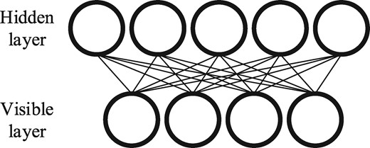
Schematic example of an RBM

RBM can be learned by using the stochastic gradient descent (SGD) on the empirical negative log-likelihood of training data, which results in the following gradients for a BBRBM (Bengio et al., 2009)

$$-\frac{\partial \hspace{0.17em}\text{log}\hspace{0.17em}p(v)}{\partial W_{\mathit{ij}}}=E_v[p(h_i|v)·v_j]-v_j^{(i)}·\mathit{sigm}(W_i·v^{(i)}+c_i)$$

(2)

$$-\frac{\partial \hspace{0.17em}\text{log}\hspace{0.17em}p(v)}{\partial c_i}=E_v[p(h_i|v)]-\mathit{sigm}(W_i·v^{(i)})$$

(3)

$$-\frac{\partial \hspace{0.17em}\text{log}\hspace{0.17em}p(v)}{\partial b_j}=E_v[p(v_j|h)]-v_j^{(i)}$$

(4)

where sigm denotes the sigmoid function $\mathit{sigm}(x)=1/(1+\text{exp}(-x))$⁠. These equations compute the expectations over all possible configurations of input data, which is difficult. A feasible solution is to estimate the expectations with a fixed number of samples. Several sampling techniques have been developed to calculate the gradients (Cho et al., 2010; Hinton, 2002; Tieleman, 2008). In this study, we choose the contrast divergence (CD) because of its simplicity. Details of the algorithms can be found in Hinton (2002).

For GBRBM, the energy function becomes:

$$E(v,h)=\sum _{i\in \mathit{vis}}\frac{{(v_i-a_i)}^2}{2{\sigma }_i^2}-\sum _{j\in \mathit{hid}}{b}_j{h}_j-\sum _{i,j}\frac{v_i}{{\sigma }_i}{h}_j{w}_{\mathit{ij}}$$

(5)

where σ_i is the standard deviation of the Gaussian noise for visible unit i. Since learning the variance is difficult with CD, we use the same strategy as in Hinton and Salakhutdinov (2006) which normalizes each feature to have zero mean and unit variance. The variance in Eq. (5) is then set to 1, and the resulted learning procedures remain the same except for that when CD is performed, the reconstructed value of a Gaussian visible unit changes from $\mathit{sigm}(W^{\prime }h+b)$ to $(W^{\prime }h+b)$⁠.

2.2 Multimodal DBN

Multimodal DBN was originally proposed to learn joint representations from image and text data (Srivastava and Salakhutdinov, 2012). In this study, multimodal DBN is used to learn cross-modality features with raw features extracted based on PPI networks and GO terms. Figure 2 gives a schematic multimodal DBN for predicting disease genes. The left and right subnetworks denote two DBNs which model PPI-based features and GO-based features, respectively. The top network is a DBN that models the joint distribution and a sigmoid activation function as the output layer for decision making.

Fig. 2.

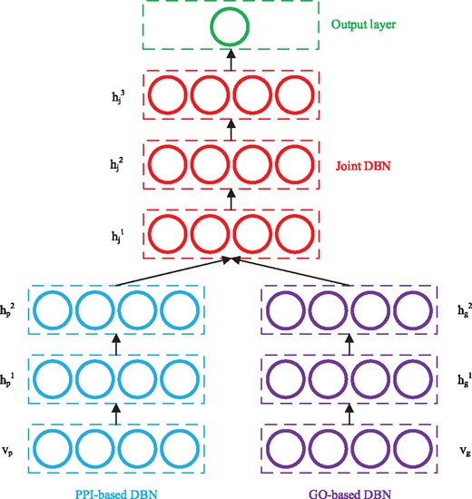
Schematic example of a multimodal DBN for disease gene prediction

According to Bengio et al. (2007), each DBN in Figure 2 can be regarded as a stack of RBMs and trained in a greedy layer-wise manner. Starting from the visible layer, every pair of adjacent layers form an RBM, which can be trained by the approach discussed in Section 2.1. In this study, the visible layers in the two sub-models use Gaussian units, and the corresponding RBMs formed by $v_p,h_p^1$ and $v_g,h_g^1$ are GBRBM. All the rest RBMs formed by adjacent hidden layers are BBRBM. Once an RBM is trained, the activation probabilities of its hidden layer are used as the input data to train the next RBM, and the DBN can be trained in this layer-wise manner. After training the two sub-DBNs, their output (hidden probabilities of the top layers) are concatenated, and the resulted representations are used as the input to train the joint DBN.

The whole model is trained in an unsupervised way, and the resulted multimodal DBN can be further analyzed by many approaches. In this study, we add an output layer with a sigmoid function to predict the probability of each disease–gene pair being associated using the cross-modality representations learned by the joint DBN.

2.3 Raw feature extraction

The input data of the multimodal DBN is the raw features of disease–gene pairs. These features are extracted from disease similarity networks and gene similarity networks. Specifically, for each sub-model, a disease similarity network and a gene similarity network are first constructed. Then, features of diseases and genes are extracted from their corresponding similarity networks, respectively, by node2vec (Grover and Leskovec, 2016), which is an algorithm that can learn features for nodes in networks. This algorithm performs random walk on a network and captures both local topological information and global structural equivalent properties to extract features. We choose node2vec because it can generate independent features which are suitable for the input of the multimodal DBN. In addition, experiments have shown that features obtained by node2vec are more informative than those of other algorithms in classification task (Grover and Leskovec, 2016).

The following two sections discuss the strategies used to construct similarity networks based on PPI networks and GO terms.

2.3.1 Similarity networks in PPI-based sub-model

In the PPI-based model, gene–gene interaction network mapped from the PPI network is regarded as the gene similarity network. This strategy is chosen because interacting proteins may have similar functions and protein interactions can reflect the functional similarities between the corresponding genes. Meanwhile, instead of constructing another gene similarity network, the topological structure of the PPI network is also valuable when extracting features with node2vec.

The disease similarity network $N_d^{\mathit{PPI}}$ is constructed according to the disease module theory. A disease module in an interactome is a subgraph consisting of genes associated with the disease (Menche et al., 2015). Let $M_1=(V_1,E_1)$ denote the disease module of disease d₁ in the interactome (gene–gene interaction network). $V=\{g_{11},g_{12},\dots ,g_{1n_1}\}$ is a set of disease genes associated with d₁, and E₁ is a set consisting of their interactions. $M_2=(V_2,E_2)$ is another disease module with similar definition. According to Ni et al. (2018), the similarity between two disease modules M₁ and M₂ can be calculated as follows:

$$\mathit{si}{m}_{\mathit{ppi}}(M_1,M_2)=\frac{\sum _{1\le s\le n_1}{F}_{M_2}(g_{1s})\sum _{1\le t\le n_2}{F}_{M_1}(g_{2t})}{n_1+n_2}$$

(6)

where $F_M(g)=\mathit{avg}(\sum _{g_i\in M}sim(g,g_i))$ measures the relations between gene g and disease module M, which is the sum of the transformed similarities between g and the genes in disease module M. Given two genes g₁ and g₂ in the PPI network, their transformed similarity is calculated by

$$\mathit{sim}(g_1,g_2)=\{\begin{array}{cc}1,\hfill & g_1=g_2\hfill \\ e^{-\mathit{sp}(g_1,g_2)},\hfill & \text{otherwise}\hfill \end{array}$$

where $\mathit{sp}(g_1,g_2)$ is the length of the shortest path between g₁ and g₂ in the PPI network. The larger the transformed similarity, the closer the relationship between g₁ and g₂.

After calculating the similarities between modules M₁ and M₂, the similarities between diseases d₁ and d₂ can be obtained by normalizing the module similarities as follows:

$$\mathit{SI}{M}_{\mathit{ppi}}^d(d_1,d_2)=\frac{2*\mathit{si}{m}_{\mathit{ppi}}(M_1,M_2)}{\mathit{si}{m}_{\mathit{ppi}}(M_1,M_1)+\mathit{si}{m}_{\mathit{ppi}}(M_2,M_2)}$$

(7)

Finally, $N_d^{\mathit{PPI}}$ is constructed by k nearest neighbors (KNN) algorithm (Cover and Hart, 1967). Specifically, edges are added to $N_d^{\mathit{PPI}}$ for each disease and its top-k most similar diseases obtained by Eq. (7). These edges are weighted by the similarity scores of their two connected diseases. In this study, k = 10 is chosen according to our previous experience (Luo et al., 2019).

2.3.2 Similarity networks in GO-based sub-model

Similar to the construction of $N_d^{\mathit{PPI}}$⁠, the GO-based similarity networks are also built by KNN algorithm, except that the similarities between diseases and genes are calculated based on GO instead of PPI network.

GO database provides a set of vocabularies to describe gene products based on their functions in the cell. Three types of ontologies are defined in GO: biological process, cellular component and molecular function. All the GO terms exist as directed acyclic graphs (DAGs) where nodes represent terms while edges represent semantic relations. In this study, we use the approach developed by Wang et al. (2007) to measure the semantic similarities of GO terms and genes.

Let $\mathit{DA}{G}_A=(T_A,E_A)$ represent GO term A, where T_A contains all the successor GO terms of A in the DAG, and E_A contains the semantic relations between A and other terms in T_A. Each term t in T_A has an S-value related to A:

$$\{\begin{array}{c}{S}_A(t)=1,\mathit{if}\hspace{0.17em}t=A\hfill \\ S_A(t)=\mathit{max}\{w_e*S_A(t^{\prime })|t^{\prime }\in \mathit{children}\hspace{0.17em}\mathit{of}\hspace{0.17em}t\},\mathit{otherwise}\hfill \end{array}$$

(8)

where w_e is the weight of the edge (semantic relations) in the DAG. Two types of semantic relations are used in the DAG: ‘is_a’ and ‘part_of’, and the corresponding w_e is set as 0.8 and 0.6, respectively, as recommended in Wang et al. (2007).

Given $\mathit{DA}{G}_A=(T_A,E_A)$ and $\mathit{DA}{G}_B=(T_B,E_B)$ for two GO terms A and B, the semantic similarity of these two terms is computed by:

$$\mathit{SGO}(A,B)=\frac{\sum _{t\in T_A\cap T_B}(S_A(t)+S_B(t))}{\sum _{t\in T_A}{S}_A(t)+\sum _{t\in T_B}{S}_B(t)}$$

(9)

The semantic similarity of one GO term $t^{\prime }$ and a set of GO terms $\mathit{GO}=\{t_1,t_2,\dots ,t_l\}$ is defined as:

$$\mathit{si}{m}_{\mathit{go}}(t^{\prime },\mathit{GO})=\underset{1\le i\le l}{\max }(\mathit{SGO}(t^{\prime },t_i))$$

(10)

Then, the functional similarity of two genes g₁ and g₂, annotated by GO term set $G{O}_1=\{t_{11},t_{12},\dots ,t_{1n_1}\}$ and $G{O}_2=\{t_{21},t_{22},\dots ,t_{2n_2}\}$⁠, is calculated by:

$$\begin{array}{c}SI{M}_{\mathit{go}}^g(g_1,g_2)=\hfill \\ \frac{\sum _{1\le i\le n_1}si{m}_{\mathit{go}}(t_{1i},G{O}_2)+\sum _{1\le j\le n_2}si{m}_{\mathit{go}}(t_{2j},G{O}_1)}{n_1+n_2}\end{array}$$

(11)

The similarity of two diseases d₁ and d₂, associated with two sets of genes $V_1=\{g_{11},g_{12},\dots ,g_{1n_1}\},\hspace{0.17em}{V}_2=\{g_{21},g_{22},\dots ,g_{2n_2}\}$⁠, is defined as:

$$\begin{array}{c}SI{M}_{\mathit{go}}^d(d_1,d_2)=\hfill \\ \frac{\sum _{1\le i\le n_1}SG(g_{1i},D{G}_2)+\sum _{1\le j\le n_2}SG(g_{2j},D{G}_1)}{n_1+n_2}\end{array}$$

(12)

where $\mathit{SG}(g^{\prime },\mathit{DG})={\max }_{1\le i\le l}(\mathit{SI}{M}_{\mathit{go}}^g(g^{\prime },g_i))$⁠.

2.3.3 Sub-model input construction

After obtaining the similarity networks, features are extracted by node2vec. Let ${\varphi }_i^p$ denote the extracted feature vector of disease i, and ${\phi }_j^p$ denote the extracted feature vector of gene j in the PPI-based model. Their concatenation, ${\psi }_{\mathit{ij}}^p=({\varphi }_i^p,{\phi }_j^p)$⁠, is the feature vector of disease–gene pair (i, j) in the PPI-based model, which is then used as the input of the PPI-based sub-DBN. Similarity, ${\psi }_{\mathit{ij}}^{\mathit{go}}$ is constructed and used as the input of the GO-based sub-DBN.

2.4 Evaluation metrics

The area under Receiver Operating Characteristics (ROC) curve (AUC) is used to evaluate the algorithms. ROC curve plots the true positive rate [TP/(TP+FN)] versus the false positive rate [FP/(FP+TN)] at different thresholds, and a larger AUC score represents better overall performance. In this study, a true positive (TP) is a known disease–gene association (positive sample) predicted as a disease–gene association, while a false positive (FP) is a non- disease–gene association (negative sample) predicted as a disease–gene association. A false negative (FN) is a positive sample predicted as negative while a true negative (TN) is a negative sample predicted as negative.

Considering that negative samples are not included in existing databases, we combine our previous study in Luo et al. (2019) and the idea of reliable negatives in Yang et al. (2012) to collect a subset of unknown samples as potential negative samples (PN). Taking the PPI-based model as an example, let ${\psi }_{\mathit{avg}}^p$ denote the average feature vector of all positive samples. For each unknown sample u, we calculate the Euclidean distance $d_u^p$ between u and ${\psi }_{\mathit{avg}}^p$⁠. The average distance is then denoted as $d_{\mathit{avg}}^p$⁠. If $d_u^p>d_{\mathit{avg}}^p$⁠, sample u is considered as a reliable negative sample. With this approach, two sets of reliable negative samples are collected from the PPI-based model and GO-based model, respectively. disease–gene pairs in the intersection of the two sets are regarded as PN. In our experiment, 4432 samples (the same as the number of positive samples) are randomly selected from PN as negative samples and the dataset contains 8864 samples in total. This random selection is performed three times to generate three sets of data.

The proposed method is evaluated in three steps. First, the whole dataset is randomly split into three subsets: training set (80%), validation set (10%) and testing set (10%). The optimized hyperparameters are determined based on the average AUC obtained from 10 randomly split validation sets. The average AUC obtained from testing sets with the optimized hyperparameters is used to evaluate the overall performance of the model. Second, dgMDL is compared with two newly developed algorithms: PBCF (Zeng et al., 2017) and Know-GENE (Zhou and Skolnick, 2016) in 5-fold cross-validation. PBCF is an MF-based algorithm and Know-GENE uses the boosted regression to predict disease–gene associations. Both of them are generic models which use similar types of data as dgMDL does. For each set of data, the cross-validation is run for five times to remove the influence of the random splitting. Associations left for testing are not used to calculate disease similarities. Third, unknown disease–gene pairs are ranked by their probabilities of being associated predicted by dgMDL. The top-10 pairs and top-10 unknown lung cancer-related genes are further studied in existing literature to evaluate the performance of dgMDL in predicting new disease–gene associations.

2.5 Hyperparameters

In this study, several hyperparameters affect the accuracy of the prediction. For the multimodal DBN, the numbers of hidden layers and the number of nodes in each hidden layer determine the architecture of the model. In our experiments, the model is found to be insensitive to the number of hidden nodes. Thus, we set the number of hidden nodes in the sub-modal and the joint-model to 256 and 512, respectively. In addition, since the performance of the model becomes stable when the numbers of hidden layers are larger than 2, we set the numbers of hidden layers to be 3 in both the sub-DBN and the joint-DBN.

Another three hyperparameters [learning rate (lr), batch size (bs) and number of epochs (ne)] determine whether the model is well trained. For lr, 0.01 is recommended for training BBRBM in Hinton (2012). In our study, we find that 0.01 is small enough to train the BBRBM. A smaller or adaptive lr barely changes the prediction accuracy. Thus, lr used for training BBRBM is set to 0.01. Meanwhile, it is recommended that lr used for training GBRBM should be one or two orders of magnitude smaller than that for BBRBM. Thus, we search lr of the GBRBM from {0.001, 0.0005, 0.0002, 0.0001}. For bs, a recommended value is usually equal to the number of the classes, and it would be better if each mini-batch contains at least one sample from each class. Considering that we only have two classes in this study and using a bs equals to two can hardly guarantee the recommendation, bs is searched from {2, 4, 8, 10}. For ne, we fix it to 30 because the performance of dgMDL becomes stable after being trained for 30 epochs. Supplementary Table S1 in the Supplementary gives the average AUC obtained from the validation sets with different combinations of lr and bs. The optimized lr for the GBRBM and bs are 0.0005 and 4, respectively.

For node2vec, the hyperparameters include: dimension of features (d); return parameter (p); in-out parameter (q); number of walks (r); length of walk (l) and context size (k). The corresponding default values recommended in Grover and Leskovec (2016) are 128, 1, 1, 10, 80 and 10, respectively. Although these hyperparameters should be changed for networks with different numbers of nodes and edges, searching all of them with brute force would be time-consuming. In our study, we do test different combinations of d, p, q and l, but the results are all worse than the ones obtained with the default values. To determine the real optimized hyperparameters used in node2vec, one might need a large amount of time on the grid search, which is not the key issue of the deep learning model. Therefore, the default values of node2vec are used in our study.

2.6 Data sources

The disease–gene association data are downloaded from the Online Mendelian Inheritance in Man (OMIM) database (Amberger et al., 2015). The latest Morbid Map at OMIM contains nearly seventy-five hundred entries sorted alphabetically by disease names, thirty-nine hundred genes and more than sixty-one hundred diseases. Each entry represents an association between a gene and a disease. Different entries are labelled with different tags [‘(3)’, ‘[]’ and ‘?’] indicating their reliabilities. To get the most reliable entries, in this study three steps are performed to preprocess the originally downloaded dataset. The first two steps are similar to the approach used in Goh et al. (2007). From the website of OMIM, diseases with tag ‘(3)’ indicate that the molecular basis of these diseases is known, which means the associations are reliable. Entries with ‘[]’ represent abnormal laboratory test values while entries with ‘?’ represent provisional disease–gene associations. At the first step, entries with the tag ‘(3)’ are selected while others are abandoned. At the second step, we classify these disease entries into distinct diseases by merging disease subtypes based on their given disorder names. For instance, 14 entries of ‘46XX sex reversal’ are merged into disease ‘46XX sex reversal’, and the 9 complementary terms of ‘Renal cell carcinoma’ are merged into ‘Renal cell carcinoma’. During the classification, string match is first used to classify adjacent entries, and then the classified results are manually verified. At the third step, 475 diseases are removed because each of them is associated with only one gene which is not associated with any other diseases. As a result, we obtain the final dataset consisting of 4432 associations between 1154 diseases and 2909 genes. All these disease–gene associations are included in Supplementary Table S2.

The PPI network is obtained from the InWeb_InBioMap database (version 2016_09_12) (Li et al., 2016a), which consists of more than 600, 000 interactions collected from eight databases. The proteins in the network are mapped to their corresponding genes to form a gene–gene interaction network. In total, there are 17429 genes in the network. GO data are downloaded from the GO database (Ashburner et al., 2000; Consortium, 2017). For genes that have no ontology information, the values of their features in the GO-based model are all 0.

3 Results

3.1 Overall performance

Figure 3 shows the average AUC obtained with the hidden representatives learned from different layers of the model. The raw feature vectors and the activation probabilities learned in each hidden layer are used to predict disease–gene associations in the testing set. The blue bars and purple bars show the AUC scores obtained from the PPI-based DBN and GO-based DBN, respectively. AUC scores obtained from the joint DBN are shown by the red bars. Clearly, the accuracy of the prediction improves when the model is continuously trained, which shows that the multimodal DBN successfully learns valuable information in different stages of the training and improves the prediction of disease–gene associations.

Fig. 3.

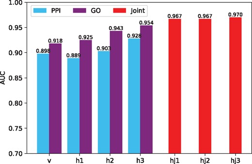
AUC of dgMDL in different layers. Among the bars correspond to the sub-DBNs (v, h1, h2 and h3), the left ones show the AUC scores of PPI-based sub-DBN and the right ones show the AUC scores of GO-based sub-DBN

3.2 Comparison with other algorithms

Figure 4 shows the ROC curves of dgMDL (red), Know-GENE (blue) and PCFM (orange) obtained with 5-fold cross-validation, respectively. dgMDL achieves an AUC of 0.969 which is the best among three competing algorithms. The AUC of Know-GENE is 0.941, which is slightly worse than that of dgMDL. PCFM ranks the 3rd with an AUC of 0.791.

Fig. 4.

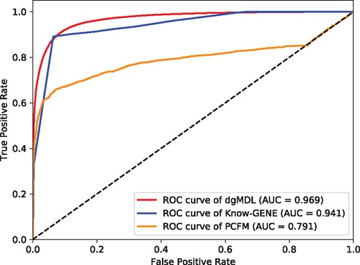
ROC curves of the three algorithms

3.3 Prediction of new disease–gene associations

To further evaluate dgMDL, we rank the unknown disease–gene pairs according to their probabilities of being associated calculated by the model. Since known disease genes are more likely to be associated with other diseases, we rank the unknown pairs of diseases and existing disease genes in this study. Meanwhile, we also rank the unknown pairs by Know-GENE and PCFM for comparison. Table 1 lists the top-10 ranked pairs of dgMDL, Know-GENE and PCFM, respectively. For dgMDL, 8 out of the 10 pairs have been studied in existing literature. While for Know-GENE and PCFM, only 3 of the 10 pairs have been studied.

Table 1.

Top-10 associations predicted by dgMDL, Known-GENE and PCFM

Disease	Gene	Supporting evidence
dgMDL
Deafness	PIK3CD	Zou et al. (2016)
Deafness	PIK3CA
Deafness	PIK3R1	Avila et al. (2016)
Diabetes	AR	Yu et al. (2014)
Deafness	PTPN11	Bademci et al. (2016)
Diabetes	SMAD4	Kim et al. (2017)
Cataract	AR
Diabetes	GATA3	Muroya et al. (2010)
Mental retardation	SMAD4	Caputo et al. (2012)
Deafness	STAT3	Wilson et al. (2014)
Know-GENE
Acne inversa familial	NLRP12
Basal cell nevus syndrome	HGF
Bladder cancer somatic	PIK3CA	Kompier et al. (2010)
Bladder cancer somatic	NRAS
Cardiofaciocutaneous syndrome	EGFR
Complement factor I deficiency	C3	Alba-Domínguez et al. (2012)
LADD syndrome	PIK3CA
Meckel syndrome	B9D1	Hopp et al. (2011)
Nevus epidermal somatic	ERBB2
Nevus epidermal somatic	RET
PCFM
Mental retardation	CLCN7
Mental retardation	PDE3A
Mental retardation	RBM12
Mental retardation	BPTF	Stankiewicz et al. (2017)
Mental retardation	TAP1
Mental retardation	LAMTOR2	Sonmez et al. (2017)
Mental retardation	DYSF
Mental retardation	TPRKB
Mental retardation	HERC1	Nguyen et al. (2016)
Mental retardation	RORC

In addition to the top-10 prediction, we test the ability of dgMDL in predicting new associated genes for a specific disease. Table 2 lists the top 10 unknown genes associated with lung cancer. 9 out of 10 pairs have been studied in existing literature. All these results demonstrate that dgMDL is valuable in predicting new disease–gene associations.

Table 2.

Top-10 susceptible lung cancer-associated genes

Gene	Supporting evidence
PTPN11	Prahallad et al. (2015)
PIK3R1	Cheung and Mills (2016)
HRAS	Kiessling et al. (2015)
GATA3	Miettinen et al. (2014)
PIK3CD
JAK2	Xu et al. (2017)
STAT3	Grabner et al. (2015)
C5	Pio et al. (2014)
SIK1	Yao et al. (2016)
PPM1D	Zajkowicz et al. (2015)

4 Conclusion

Integrating multiple types of data with machine learning model is a challenging task, especially for predicting disease genes where the number of known associations is limited. In this study, we have proposed a method to predict disease–gene associations with the cross-modality features obtained by multimodal DBN. The deep learning model learns joint representations from raw features extracted from PPI-based similarity networks and GO-based similarity networks. Results show that the proposed method is overall more accurate than the competing algorithms. Further analysis of the top-10 disease–gene pairs and top-10 lung cancer-related genes also reveal the potential of dgMDL in predicting new disease genes. The current model integrates two types of data. It is possible that a gene is not included in any of these data, and its associations cannot be correctly predicted. In the future, more types of data should be integrated by the multimodal DBN, such as disease-disease associations, protein domain and sequence information, to solve this issue and improve the prediction accuracy.

Acknowledgements

The authors thank Dr Hongyi Zhou for explaining the functional association strength calculated in Know-GENE.

Funding

This work was supported by the Natural Science and Engineering Research Council of Canada (NSERC); China Scholarship Council (CSC); the National Natural Science Foundation of China [Grant No. 61772552, 61571052]; and the Science Foundation of Wuhan Institute of Technology [Grant No. K201746].

Conflict of Interest: none declared.