


Abstract
Protein activity is a significant characteristic for recombinant proteins which can be used as biocatalysts. High activity of proteins reduces the cost of biocatalysts. A model that can predict protein activity from amino acid sequence is highly desired, as it aids experimental improvement of proteins. However, only limited data for protein activity are currently available, which prevents the development of such models. Since protein activity and solubility are correlated for some proteins, the publicly available solubility dataset may be adopted to develop models that can predict protein solubility from sequence. The models could serve as a tool to indirectly predict protein activity from sequence. In literature, predicting protein solubility from sequence has been intensively explored, but the predicted solubility represented in binary values from all the developed models was not suitable for guiding experimental designs to improve protein solubility. Here we propose new machine learning (ML) models for improving protein solubility in vivo.
We first implemented a novel approach that predicted protein solubility in continuous numerical values instead of binary ones. After combining it with various ML algorithms, we achieved a R2 of 0.4115 when support vector machine algorithm was used. Continuous values of solubility are more meaningful in protein engineering, as they enable researchers to choose proteins with higher predicted solubility for experimental validation, while binary values fail to distinguish proteins with the same value—there are only two possible values so many proteins have the same one.
We present the ML workflow as a series of IPython notebooks hosted on GitHub (https://github.com/xiaomizhou616/protein_solubility). The workflow can be used as a template for analysis of other expression and solubility datasets.
Supplementary data are available at Bioinformatics online.
1 Introduction
Escherichia coli is a bacterium commonly used in genetic engineering to express recombinant proteins (Chan et al., 2010), which is a pivotal process in biotechnology. Producing some proteins in E.coli was, however, inefficient in industrial setting, resulting from low activity of the recombinant proteins. As biocatalysts and therapeutic agents, proteins with high activity have lower unit production cost. Developing biocatalysts with high activity has thus become an important goal for further development of many biocatalytic processes.
Some experimental strategies in vivo can improve the expression of recombinant proteins, such as using suitable promoters, optimizing codon usage, or changing culture media, temperature and/or other culture conditions (Idicula-Thomas and Balaji, 2005; Magnan et al., 2009). Such empirical optimizations have, however, been time-consuming and expensive. Moreover, experiments often fail due to opaque reasons. A generic solution is highly desired for enhancing the heterologous protein overexpression and may be ultimately provided by using a computational model that can predict activity of any enzyme accurately from its amino acid sequence and other input information. Developing such model would require a large dataset which contains at least two columns, protein sequence and activity. No such dataset is currently available, because conventional protein engineering was driven by chasing high activity, which has provided very little information on protein sequence. For instance, most proteins with low or intermediate activity values were discarded without their sequence being revealed. It is currently prohibitively expensive to generate a complete, large dataset for protein activity, due to technical limitations.
A compromised solution is to predict protein activity by using solubility of the protein as a proxy, because (i) activity and solubility are correlated for some proteins (Zhou et al., 2012), and (ii) there is a relatively large dataset available for solubility as solubility data from different proteins can be pooled together. Until now, a number of machine learning (ML) predictors have been developed to address the interconnection between protein solubility and amino acid sequence. The prediction for protein solubility from amino acid sequence was first proposed by Wilkinson and Harrison (1991). A simple regression method was used by them to achieve high accuracy (0.88) by using several features of 81 protein sequences, such as hydrophilicity, molecular weight and averaged surface charge. The accuracy was improved by logistic regression to 0.94 based on a small database with 212 proteins (Diaz et al., 2010). Support vector machine (SVM) is a core ML classification method that has achieved competitive performance in this field. With SVM, Idicula-Thomas et al. (2006) analysed 192 proteins with an unbalanced correlation score filter, which achieved an accuracy of 0.74 by using physicochemical properties, mono-peptide frequencies, dipeptide frequencies and reduced alphabet set as features. These datasets are, however, not large enough to generate correlations that can be widely applied (Idicula-Thomas and Balaji, 2005). Molecular weight, isometric point and amino acid composition were used as inputs to build a SVM model by Niwa et al. (2009), who for the first time generated and studied a dataset that contained more than 1000 proteins. Prediction of protein solubility was subsequently conducted with SVM based on databases with 2159 proteins (Agostini et al., 2012) and 5692 proteins (Xiaohui et al., 2014). Besides, decision tree (Christendat et al., 2000; Goh et al., 2004; Rumelhart et al., 1985), Naïve Bayes (Smialowski et al., 2007), random forest (Fang and Fang 2013; Hirose et al., 2011), gradient boosting machine (Rawi et al., 2017) and some computational methods combining multiple ML models have been utilized to predict if a protein is soluble or not by using their primary sequence. In addition, several software and web servers have been developed for protein solubility prediction, including ESPRESSO (Hirose and Noguchi, 2013), Pros (Hirose and Noguchi, 2013), SCM (Huang et al., 2012), PROSOII (Smialowski et al., 2012), SOLpro (Magnan et al., 2009) and PROSO (Smialowski et al., 2007). Some of the predictors available online are introduced below. ESPRESSO selects features by using Student’s t-test filter and trains a model by SVM and another sequence pattern recognition-based method. Pros implements random forest with Student’s t-test as filter and random forest as wrapper. PROSOII is a two-layer model using a Parzen window in the first layer and logistic regression in both layers.
Various databases were also utilized in the previous studies, whereas eSol database (Niwa et al., 2009) is a unique one, which has a relatively large size and continuous values of solubility, ranging from 0 to 1. A brief summary of how solubility values in eSol database were obtained is provided here. Proteins were produced in vitro by using cell-free protein expression technology and plasmids carrying open reading frame (ORF) from complete E.coli ORF library (ASKA library) (Kitagawa et al., 2005). Synthesized proteins were fractionated into soluble and insoluble fractions by using centrifugation, and the proteins in both fractions were quantified by using SDS-PAGE. Solubility was defined as the ratio of protein quantity of the supernatant to the total protein quantity. Comparison of model performances using this database is summarized in Table 1. All the ML models developed based on this database, however, only predicted whether a protein was soluble or insoluble (outputting binary values), which was not useful in guiding protein engineering, because even a substantial increase in solubility may not turn the status from ‘insoluble’ to ‘soluble’ and thus be falsefully viewed as useless by the model. Moreover, it is challenging to select several proteins with highest solubility to conduct experiments because there are too many proteins with the same value of solubility (i.e. 1) in a large dataset. Moreover, in the process of grouping the proteins, all the previous works discarded data points whose protein solubility was between 0.3 and 0.7.
Performance of published methods based on eSol database
| Method | Size | Accuracy | References |
|---|---|---|---|
| Random forest | Total: 1918 | 0.84 | (Fang and Fang, 2013) |
| Soluble: 886 | |||
| Insoluble: 1032 | |||
| 1. SVM | Total: 1625 | 0.81a | (Samak et al., 2012) |
| 2. Random forest | Soluble: 843 | ||
| 3. Conditional inference trees | Insoluble: 782 | ||
| 4. Rule ensemble | |||
| Decision tree | Size: 1625 | 0.75 | (Stiglic et al., 2012) |
| Soluble: 843 | |||
| Insoluble: 782 | |||
| SVM | Size: 2159 | N/A | (Agostini et al., 2012) |
| Soluble: 1081 | |||
| Insoluble: 1078 | |||
| SVM | Size: 3173 | 0.80 | (Niwa et al., 2009) |
| Soluble: >0.7 | |||
| Insoluble: <0.3b |
Value estimated from the figure in the reference.
Proteins with solubility higher than 0.7 are labelled as soluble and lower than 0.3 are labelled as insoluble.
In addition, adequate volume of data is key to develop useful models by using ML. In biotechnology field, generating and collecting large amount of data is; however, time-consuming and expensive, resulting in much smaller dataset than other fields such as facial recognition. Generative Adversarial Networks (GANs) (Goodfellow et al., 2014), a state-of-the-art data augmentation algorithm in artificial intelligence (AI), have been utilized to enlarge data in both computer vision and biological fields. For example, GANs have been used to generate mimic DNA sequences for optimizing antimicrobial properties of recombinant proteins (Gupta and Zou, 2018) and to access the local geometry by local coordinate charts (Qi et al., 2018). To date, the data argumentation algorithms have not been applied to the problem of protein solubility.
In this study, we built models that can predict protein solubility in numerical values that span from 0 to 1, which would allow fair evaluation of a proposed mutation to a protein even when the resulting improvement is small. We compared various model-building techniques which used this new output format, and found SVM performed the best, achieving a R2 of 0.4115. Moreover, we hypothesized that data augmentation algorithms might alleviate the problem that biotechnology applications do not have sufficient data for developing ML models. We attempted to use GANs to improve the prediction performance of the SVM model by generating artificial data.
2 Materials and methods
2.1 Protein database
All the proteins used in the study were downloaded from eSol database (Niwa et al., 2009). Here, the solubility refers to the ratio of soluble protein to the total protein, not the limit concentration above which solute precipitates in the solvent. Many recombinant proteins, when overexpressed in a heterologous host, become insoluble because of misfolding. The information about protein solubility and the corresponding name of genes were included in the eSol database. According to the name of genes, protein sequence for each protein was searched in NCBI and matched with the protein solubility. We used all the proteins from the database, unless the proteins contain no sequence information, or poorly determined sequence (e.g. containing N instead of A, T, C or G, or multiple stop-codons). Supplementary Table S1 summarized the reasons that 26 data points were excluded in our study. After excluding 26 proteins in total, the data size used in our study was 3147.
2.2 Features
Different features were extracted from sequences of proteins by using protr package (Xiao et al., 2014) within R software, which generates various numerical representation schemes. In our study, the description of features is listed in Table 2 according to different descriptors in protr package.
Description of different descriptors in protr package of R software
| Descriptors | Description |
|---|---|
| extractAAC | composition of each amino acid |
| extractPAAC | hydrophobicity, hydrophilicity and side chain mass |
| extractAPAAC | hydrophobicity, hydrophilicity and sequence order |
| extractMoreauBroto | normalized average hydrophobicity scales, average flexibility indices, polarizability parameter, free energy of solution in water |
| extractMoran | normalized average hydrophobicity scales, average flexibility indices, polarizability parameter, free energy of solution in watera |
| extractGeary | normalized average hydrophobicity scales, average flexibility indices, polarizability parameter, free energy of solution in watera |
| extractCTDC | hydrophobicity, normalized van der Waals volume, polarity, polarizability, charge, second structure, solvent accessibility |
| extractCTDT | percentage of position of attributes in extractCTDC |
| extractCTDD | distribution of attributes in extractCTDT |
| extractCTriad | protein–protein interactions including electrostatic and hydrophobic interactions |
| extractSOCN | Schneider-Wrede physicochemical distance matrix and Grantham chemical distance matrix |
| extractQSO | Schneider-Wrede physicochemical distance matrix and Grantham chemical distance matrixb |
Different calculation methods are used for extractMoreauBroto, extractMoran and extractGeary using the same attributes listed above.
Different calculation methods are used for extractSOCN and extractQSO using the same attributes listed above.
2.3 Training flowsheet
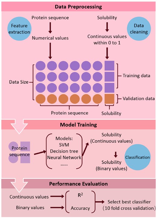
Data pre-processing is a very important part in data mining, which transfers raw data into a well-organized dataset that can be taken as inputs in model training. Only sequence and protein solubility were retrieved from the original dataset. Protein sequence was then transformed into numeric values (features) by using extractAAC descriptor from Table 2. The values of protein solubility which were to be higher than 1 were converted into 1 as the protein solubility represents the ratio of supernatant protein to the total protein. Some experimental errors caused the values of protein solubility recorded higher than 1. After cleaning the dataset, the table recoding the dataset has 3147 rows and several columns whose number depends on the descriptors used. Each row means one data point or one protein. The last column stores protein solubility data, and each of the other columns stores values of one descriptor.
Training ML models for protein solubility prediction included several steps (as shown in Fig. 1). The inputs and outputs of ML models were protein sequence and protein solubility respectively. For training ML models, 90% of the original dataset (2833 proteins) were used and the remaining dataset were validation data which can be used to evaluate the performance of each model. After model training, all the evaluation metrics were calculated with 10-fold cross-validation to compare the performance of different ML models. The 10-fold cross-validation is a technique to partition the original dataset into 10 equal-size parts. And each part has similar proportion of samples from different classes. In the 10 subsamples, one subsample is taken as validation data to test the model and the other data is used as training data to train the model. The accuracy and R2 are the average of all the cases. For the data augmentation, 75% of the original data (2364 proteins) were used as training data to train the four data augmentation algorithms, which then generated the same size of artificial data (2364 proteins). Then the ML models were trained again on the doubled training data including both the original training data and the generated data. Subsequently, a new value of R2 was calculated by the validation data which were held out in the training process. The improvement of R2 represents the performance of data augmentation.
Workflow of model training used in our study
2.4 ML models
Seven supervised ML algorithms were applied to our dataset: logistic regression, decision tree, SVM, Naïve Bayes, conditional random forest (cforest), XGboost and artificial neural networks (ANNs). The first five models were used by implementing the corresponding packages in R and the last two models were utilized by applying the corresponding libraries in Python. All the hyperparameters can be tuned by changing the arguments in the functions. For binary values of solubility, classification algorithms were used and for continuous values of solubility, regression algorithms were applied.
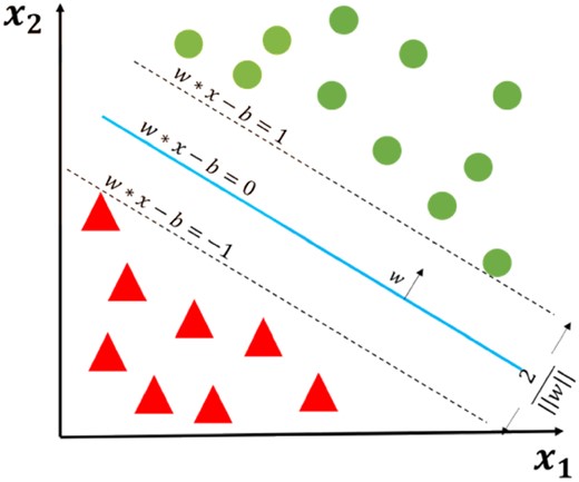
Maximum-margin hyperplane for a SVM trained with samples with two classes (Note: This is an illustration of basic SVM classification algorithm and we used a regression version in our study.)
2.5 Tuning SVM
Among the ML models used to predict the protein solubility, SVM achieved the best performance. Therefore, SVM was chosen for further optimization to achieve higher prediction R2 by tuning all parameters (Package e1071 in R software was used to implement SVM model). Different kernels (representing different functions) and three parameters (cost, gamma and epsilon) in SVM were tuned. Cost is the regularization parameter that controls the trade-off between achieving a low training error and a low testing error. Cost can also be interpreted as the extent we penalize the SVM when data points lie within the dividing hyperplanes. Larger cost means fewer points are within the dividing hyperplanes and the space between two dividing hyperplanes is small, which also indicates that the unseen points are difficult to be separated because the data points belonging to two categories are too close to each other. On the contrary, lower cost gives larger margin and higher error for training data. Epsilon is a margin of tolerance where no penalty is given to errors. Larger epsilon means less penalty to errors. Gamma is a parameter in the function of radial basis kernel, which indicates the threshold to determine if two points are considered to be similar. Gamma controls the standard deviation of the Gaussian function of radial basis kernel.
2.6 Data augmentation algorithms
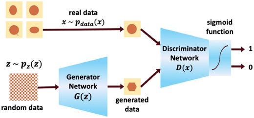
GANs are an emerging AI algorithm and have been used for data augmentation in this work. There are two main models within GANs, Generator Neural Network and Discriminator Neural Network. The generative model G takes random data z from probability distribution p(z) as input. The discriminative model D takes data generated from generative model G and real data from the training dataset as inputs and distinguishes whether the data are artificial or real. The training process is an adversarial game with backpropagation between two networks (Fig. 3).
The workflow of training GANs
With the development of AI algorithms for data augmentation, other algorithms based on GANs have also been developed, which enhanced the performance of GANs to some extent. CGAN is the conditional version of GANs, which generates mimic data with class labels (Mirza and Osindero, 2014). WGAN uses Wasserstein distance metric rather than Jensen-Shannon distance metric used in GANs when cross-entropy is calculated (Arjovsky et al., 2017). The cross-entropy loss is a measurement of the ability of the discriminator to distinguish real data and generated data. Wasserstein distance measures the minimum cost to make the distribution of generated data more similar to that of real data, with the critic function in the discriminator model. WCGAN is the conditional version of the Wasserstein GANs (Gulrajani et al., 2017). Moreover, some architectures of CGAN and WCGAN show great promise to explore datasets with labels, which both generate mimic data similar to real data and explore the relationship between features and labels. For the GANs with conditions, the relationship between features and labels was studied by constraining the labels of the generated data to be the expected values.
2.7 Evaluation metrics
The definition of TP, TN, FP and FN for binary values of solubility
| Predicted solubility from models | |||
|---|---|---|---|
| Actual solubility from experiments | Solubility = 1 | Solubility = 0 | |
| Solubility = 1 | TP | FN | |
| Solubility = 0 | FP | TN | |
| Predicted solubility from models | |||
|---|---|---|---|
| Actual solubility from experiments | Solubility = 1 | Solubility = 0 | |
| Solubility = 1 | TP | FN | |
| Solubility = 0 | FP | TN | |
We also evaluated the model performance by using coefficient of determination (R2) calculated from predicted and actual solubility values. Computing R2 can only be done by using continuous values our models generated.
3 Results
3.1 Develop models that output continuous numerical values
We used continuous values of protein solubility to train ML models, which we set to output continuous values instead of binary ones. We have trained seven distinct models and two different evaluation criteria (accuracy and R2) were recorded in Table 4. The prediction performance of the ML models was compared using R2. The accuracy was measured to explore the influence of choosing cut-off thresholds on the value of accuracy. For the purpose of calculating the accuracy, we converted the continuous values of predicted solubility into binary ones by using 0.44 (median value of the solubility data of our database) as cut-off threshold because the data above and below median exhibit same sizes. SVM showed the best prediction performance among all the ML models according to the value of R2 (Table 4). The tuned SVM parameters were listed in Supplementary Table S2 and Supplementary Figure S1. After plotting the correlation between the R2 versus cost, epsilon, or gamma, optimized values were found (0.86, 0.031 and 0.205 for cost, gamma or epsilon, respectively). The R2 indicates how well our regression model explains all the variability of the protein solubility around its mean. To evaluate our model in a more comprehensive way, we performed the analysis of variance (ANOVA) to the SVM model with the best prediction performance and the results of ANOVA are shown in Table 5. In the table, other evaluation metrics of our regression model of SVM are also provided. For example, the mean squared error, measuring the average of the squares of the errors, is 0.0639. In addition, the F statistic of 36.9342 is much higher than 1, which shows our regression model is statistically significant.
Performance of different ML models
| Model | Accuracy | R 2 | |
|---|---|---|---|
| Continuous values of solubility | Binary values of solubility | Continuous values of solubility | |
| Logistic regression | 0.6372 | 0.6868 | 0.2507 |
| Decision tree | 0.6734 | 0.6750 | 0.2459 |
| SVM | 0.7538 | 0.7001 | 0.4115 |
| Naïve Bayes | 0.6674 | 0.6979 | 0.2376 |
| cforest | 0.7055 | 0.7123 | 0.3764 |
| XGboost | 0.7052 | 0.7103 | 0.3997 |
| ANNs | 0.6632 | 0.7086 | 0.2029 |
Results of ANOVA test
| Source | Degrees of freedom | Sum of squares | Mean squares | F |
|---|---|---|---|---|
| Model | 19 | 44.8500 | 2.3605 | 36.9342 |
| Error | 784-19-1 | 48.8285 | 0.0639 | |
| Total | 784-1 | 93.6784 |
| Source | Degrees of freedom | Sum of squares | Mean squares | F |
|---|---|---|---|---|
| Model | 19 | 44.8500 | 2.3605 | 36.9342 |
| Error | 784-19-1 | 48.8285 | 0.0639 | |
| Total | 784-1 | 93.6784 |
For comparison, we also trained the models by using the conventional approach, which converted continuous actual solubility values into binary ones BEFORE model training. Though using continuous values did not always improve model prediction performance, it improved SVM model and made it to be the best one, in terms of both accuracy and R2 (Table 4).
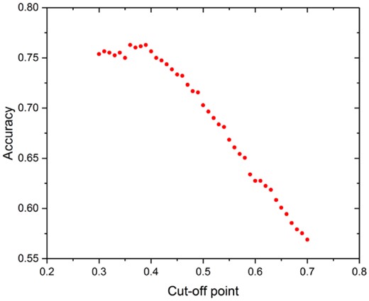
Cut-off points were used to transfer continuous values of solubility to binary values for model evaluation. How to choose the cut-off threshold substantially affects accuracy. Here we did a simple optimization of the threshold with maximizing the accuracy as the objective. When the cut-off threshold was too low (<0.3) or too high (>0.7), the accuracy would be very high, but such accuracy was not useful because almost all the proteins would be classified either as soluble or insoluble proteins. We varied the threshold from 0.3 to 0.7 with step size of 0.01 and calculated the SVM model prediction accuracy. From Figure 4, the highest accuracy (0.7628) was obtained when the cut-off point was 0.36 or 0.39. Therefore, 0.39 was randomly selected from those two values and was used in the following analysis. Although this optimization did not substantially improve SVM model prediction accuracy, the results showed that the threshold can substantially change the accuracy (Fig. 4). In the previous study using the same database with us (Fang and Fang, 2013; Samak et al., 2012), two thresholds 0.3 and 0.7 were used, which divided proteins with solubility lower than 0.3 as insoluble and proteins with solubility higher than 0.7 as soluble. The proteins with solubility within 0.3–0.7 were discarded. The method of dividing whether the proteins were soluble affected the accuracy significantly and was different from our approach. We first used one threshold 0.44 and modified it within the range 0.3–0.7 to observe the change of accuracy, whereas they used two thresholds 0.3, 0.7 and discarded the proteins with solubility between 0.3 and 0.7. Since it is arbitrary to choose a cut-off threshold, accuracy based on the cut-off threshold is intrinsically subjective. With our new methods and the resulting continuous model output values, we call for using the coefficient of determination (R2) as the model evaluation metric, which does not require any cut-off threshold. We used the R2 as the sole evaluation metric in the rest of this study.
Effect of cut-off threshold on SVM prediction accuracy
3.2 Attempt to improve model performance by optimizing data pre-processing
To further improve SVM model prediction performance, we evaluated all the available algorithms that convert amino acid sequence into numerical values. This step is critical as it extracts a fraction of information (usually only a small fraction, termed as features) from the sequence data, and feeds it to the model-training algorithms. Since most information in raw data was discarded here, avoiding loss of critical information by using a better algorithm may improve the model performance. It turned out that the best was the extractAAC descriptor that simply converted sequence into amino acid composition, and that we used in prior sessions of this study (Table 6).
Performance of different sequence descriptors by SVMa
| Descriptors | R 2 | Data dimension |
|---|---|---|
| extractAAC | 0.4108 | 20 |
| extractPAAC | 0.3564 | 50 |
| extractAAC+extractPAAC | 0.3719 | 70 |
| extractAPAAC | 0.3049 | 80 |
| extractMoreauBroto | 0.0806 | 240 |
| extractMoran | 0.0542 | 240 |
| extractGeary | 0.0562 | 240 |
| extractCTDC | 0.2484b | 21 |
| extractCTDT | 21 | |
| extractCTDD | 105 | |
| extractCTriad | 0.0650 | 343 |
| extractSOCN | 0.1647 | 80 |
| extractQSO | 0.3224 | 100 |
The description of each descriptor is shown in Table 2.
The R2 is the result combining extractCTDC, extractCTDT and extractCTDD.
3.3 Attempt to improve model performance by using data augmentation
In the first attempt, four versions of GANs were trained for 500 iterations to generate the artificial data, which were used together with the original data to train ML models by using SVM. This attempt, however, failed to improve the model performance, as R2 was not increased (Supplementary Table S3). Figures of protein sequence after dimensionality reduction by principal component analysis (PCA) and protein solubility were shown in Supplementary Figures S2 and S3. PCA can generate a lower-dimensional projection of the data and preserve the maximal data variance. Three components with highest variance were retained after projecting our features with 20 dimensions for data visualization, and they represented the three dimensions in Supplementary Figures S2 and S3. Different colours represent different values of solubility from 0 to 1. Over iterations, the quality of data generated by GANs improved (Supplementary Fig. S3), which showed GANs were implemented correctly. By comparing the performance of four versions of GANs (Supplementary Table S3), GANs and CGAN had better performance among the four versions of GANs. In addition, GANs surpassed CGAN according to the comparison between the original data and the generated data from GANs and CGAN (Supplementary Fig. S2). Therefore, GANs were explored for more iterations.
In the second attempt, we increased the number of iterations from 500 to 5000. At the end of each 100 iterations, the generated data were used together with the original data to train the SVM model. There were 50 values of R2 corresponding to 50 sets of exported generated data after we train GANs for 5000 iterations. The highest R2 among the 50 values was recorded for each training dataset (Supplementary Table S4). In Supplementary Table S4, suffixes 1, 2 and 3 represent three randomly selected training datasets from the original dataset. For each training dataset, the comparison of SVM model performance between original data and data including generated data was conducted. There was, however, no improvement of prediction performance after applying data augmentation algorithms.
Therefore, the generated data was not used for training the ML models in other sections of our study. Optimization for GANs or other data augmentation algorithms will be explored further in future work.
4 Discussion
4.1 Predict protein solubility with continuous values
In this study, we developed a new model that can use amino acid sequence to predict protein solubility in continuous values from 0 to 1, which would help improve solubility of recombinant proteins through protein engineering. Having model output in such format also enables us to use coefficient of determination (R2) as a metric to evaluate model performance, which does not depend on a subjective threshold to determine if a protein is soluble or insoluble. In literature, all the studies used such threshold(s) to convert continuous values of protein solubility in eSol database into binary values.
The R2 of our model may be improved further in three aspects. First, the descriptors we used to transfer amino acid sequence into numerical values may not include complete information for the sequence. For example, physical properties and secondary structure can be added as the features for improving the model performance. Second, the quality and quantity of the data points collected in the eSol database may not be enough to train the ML models effectively. More data can be collected by experiments or generated by data augmentation algorithms to enlarge the dataset. Finally, the R2 may be limited by using protein sequence alone for the prediction of protein solubility. Other elements can be included to further enhance the model performance such as pH and temperature in the process of expressing the proteins.
With continuous values of solubility, we will study how to use a developed model to guide experiments in the future. First, we will use statistical tools to determine the minimal performance of a model (in terms of R2) required to conduct a meaningful in silico screening of protein mutants—the average quality of selected mutants should be substantially higher than that of the initial pool of mutants. The next step is to validate the model prediction by selecting a number of proteins with high predicted solubility and measuring their actual solubility through experiments. We can generate the pool of mutants for in silico screening by randomly introducing mutants to a model protein. However, binding of substrate/co-factor and catalytic active site may be damaged by such random mutation, which would influence the catalytic function. Therefore, mutation of residues responsible for binding substrates and the catalytic activity will be avoided. Then sensitivity analysis will be conducted to determine how many mutations should be made to improve protein solubility substantially. The model we developed in this study laid the foundation for such future works, which cannot be done by using any existing models.
4.2 Enlarge dataset by data augmentation algorithms
Despite that GANs have improved ML in many applications; it failed to build better models in this case. There may be two reasons for the undesired results. First, the parameters of GANs or the architecture of the generator and the discriminator were suboptimal, so the quality of the generated data was poor. To improve GANs, we plan to conduct more optimizations of GANs parameters, such as learning rate of the generator and the discriminator. Second, model prediction performance is strongly influenced by the quality of dataset, so the quality of the dataset we used may limit us from developing better models. In this case, GANs can be tried for a part of the original dataset only including specific groups of proteins with acceptable prediction performance.
Acknowledgements
We thank Dr Wee Chin Wong, Dr Yun Long for technical discussions and Mr Shen Yifan for assistance.
Funding
This work was supported by Ministry of Education (MOE) Research Scholarship, MOE Tier-1 grant [R-279-000-452-133] and National Research Foundation (NRF) Competitive Research Programme (CRP) grant [R-279-000-512-281] in Singapore.
Conflict of Interest: none declared.
References

