


Abstract
The association of splicing signatures with disease is a leading area of study for prognosis, diagnosis and therapy. We present a novel fast-performing annotation-dependent tool called SCANVIS for scoring and annotating splice junctions (SJs), with an efficient visualization tool that highlights SJ details such as frame-shifts and annotation support for individual samples or a sample cohort.
Using publicly available samples, we show that the tissue specificity inherent in splicing signatures is maintained with the Relative Read Support scoring method in SCANVIS, and we showcase some visualizations to demonstrate the usefulness of incorporating annotation details into sashimi plots.
https://github.com/nygenome/SCANVIS and https://bioconductor.org/packages/SCANVIS.
Supplementary data are available at Bioinformatics online.
1 Introduction
The association of splicing defects with disease and variants is an ongoing area of research. Some splicing analysis tools operate independently from annotation (Li et al., 2018; Wang et al., 2018) which, while allowing for novel discoveries, lack details such as annotation support or frame shifts that can help infer functional consequences (e.g. protein truncation). Integrative Genomics Viewer IGV (Robinson, 2011) is a popular tool for creating interactive sashimi plots, but these do not visually delineate SJs supported by annotation from those that are not, and does not allow for the merging of a cohort of samples into one representative figure. To address some of these shortcomings we developed SCANVIS, an R-based tool that scores and annotates SJs with gene names, junction type and frame-shifts. It has a visualization function for generating static sashimi plots with annotation details differentiated by color and line types which can be overlaid with any available variants and read profiles. Samples in one cohort can also be merged into one figure for quick contrast to another cohort.
2 Materials and methods
SCANVIS requires two main inputs to score and annotate a sample: annotation and SJs. Annotation details from a GTF file of choice can be extracted into a SCANVIS-readable object using the annotation function in our software. Required SJ details are chromosome, start/end coordinates and junction read support as derived by an alignment algorithm of choice. In our analyses we used human gencode v19 and SJ details generated by the STAR aligner Dobin et al. (2013). SCANVIS processes one sample at a time and annotates each SJ in the samples with (i) a Relative Read Support (RRS) score, (ii) the RRS genomic interval and (iii) names of gene/s that overlap the SJ. Unannotated SJs (USJs) are further described by (iv) frame-shifts and (v) junction type, this being either exon-skip, alt5p, alt3p, IsoSwitch, Unknown or Novel Exon (NE). USJs described as IsoSwitch are SJs that straddle two mutually exclusive isoforms while Unknown USJs are contained in annotated intronic regions. A RRS genomic interval is defined as the minimal interval containing at least one gene overlapping the query SJ and at least one annotated SJ (ASJ). The RRS score is the ratio of x to x + y, where x is the query junction read support and y is the median read support of ASJs in the RRS genomic interval. This approach keeps RRS free from undue influence of USJs which tend to be frequent, have poor read support and may be alignment artifacts. Once all SJs are scored and annotated, SCANVIS looks for potential NEs defined by USJs coinciding in annotated intronic regions. NEs are scored by the mean RRS of all SJs landing on the NE start/end coordinates. If the alignment BAM file is accessible, users may optionally supply this and SCANVIS will compute an additional Relative Read-Coverage (RRC) score for NEs. This is defined as c/(c5+c+c3) where c is the mean NE read coverage, and c5 and c3 are mean read coverages for flanking regions, both defined as intervals 0.2 times the NE interval.
3 Results
We ran SCANVIS on 3706 and 4082 samples from The Cancer Genome Atlas (TCGA) and the Genotype-Tissue Expression project (GTEx) respectively, spanning 9 cancers and 14 tissue types (Supplementary Fig. S1). Using PCA and t-SNE plots (Supplementary Figs S3/S4) computed on RRS scores of the top 5000 most variable SJs (see Supplementary Fig. S2 for variance distribution), we observed good tissue separation for both cohorts. Using 1528 SJs intersecting in the top 5000 GTEx and TCGA SJs, tSNE/PCA plots computed on both cohorts (Supplementary Fig. S4, top) show more tissue than cohort separation. Figures computed on skin and thyroid samples only (Supplementary Fig. S4, bottom) show TCGA thyroid cancers clustering with GTEx thyroid samples, indicating that the local-based RRS scores retain tissue specificity and are not susceptible to batch effects. Next we trained and tested linear kernel Support Vector Machines (SVMs) using 10-fold cross-validation executed 20 times for each cohort tissue, with the top 500 variable SJs selected as model features for each iteration (variance computed over training samples). AUC scores (area under ROC curves) were 0.98 and higher for all tissue/cancer types (Supplementary Fig. S2) confirming that RRS scores retain tissue specific signatures.
The visualization tool is arguably the most useful component of SCANVIS, allowing users to quickly generate static sashimi plots overlaid with variants and read coverage for multiple samples. Arc line widths and heights relate to RRS scores and read support (log-scale) respectively, with RRS or read support shown for any USJs. ASJs are visually separated from USJs (grey versus other colors respectively) with dotted arcs indicating any USJ frame-shifts. SCANVIS includes a function to map SJs to variants so that when variant-mapped SJs are supplied to the visualization tool, variants co-occurring with SJs in the plotted region are shown as black dots (single point mutations) or black lines (indels). An example of this is shown in Figure 1 where we see the splice variant chr4: 106307724; C>A located at the start of an exon that is skipped (red arc) in PPA2 for a TCGA lung squamous cell carcinoma. Read profiles are plotted when the BAM file is supplied, allowing users to explore NE read coverage. Figure 1 shows a SCANVIS plot for the gene PLEKHA6 for a glioblastoma TCGA sample, with the read coverage (inverted black profile) indicating support for 4 NE intervals (see inserts in Fig. 1). While these are novel with respect to human gencode v19, they align to exons found in recent GRCh38 human reference gencode versions (Supplementary Fig. S5), validating this NE detection method. The SCANVIS visualization tool can also accept multiple samples to generate one representative figure over the samples, thereby allowing users to quickly contrast splicing signatures across cohorts. When merging samples, SCANVIS collects the union of all SJs and computes the mean (or optionally the median) RRS and SJ read support over the samples to derive one representative sample for visualization. If the SJs are variant-mapped, mutations are counted across the samples and any recurrent mutations are plotted as a stick-and-ball marker (also known as lollipop plots) showing the number of samples hosting the variant (see software documentation for examples).
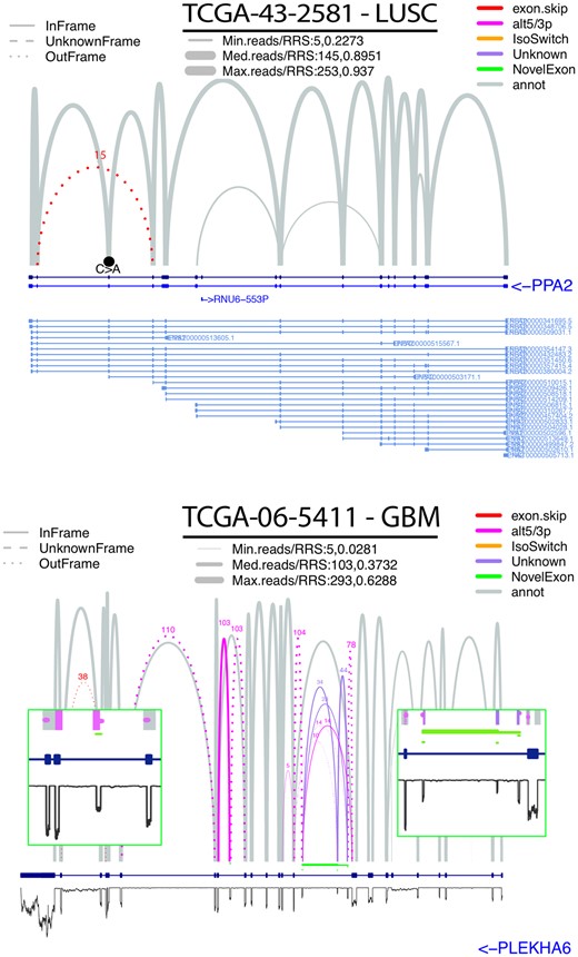
SCANVIS visualizations. Top figure shows a SCANVIS plot of the pyrophosphatase gene PPA2 of a Lung Squamous Carcinoma (LUSC) sample from TCGA with a frame-shifting exon skipping event (red arc) and the splice variant chr4: 106307724; C>A (black point) located at the start of the skipped exon. Bottom figure shows a SCANVIS plot of the pleckstrin homology domain (PLEKHA6) with splicing signatures overlaid with read coverage for a glioblastoma (GBM) sample. Here we see a number USJs coinciding in annotated intronic regions, leading SCANVIS to flag a number of NE intervals (marked in green). These align with peaks in the read coverage, none of which coincide with the coordinates of annotated exons
4 Discussion
Determining which genes harbor which splicing alterations are critical details to functional splicing analyses. SCANVIS was developed to prescribe such details, along with efficiently generated visualizations to assist in this process. It is fast, processing a sample with 170 K SJs on a 1.6 G MacBook Air 2015, macOS Sierra 10.12.6 (a 1.6GHz processor with memory 8GB 16000 MHz DDR3) in just under 6 min. We used SCANVIS extensively to analyze many in-house samples, and we hope that in making this tool accessible to the community, researchers can dig deeper into splicing signatures with more transparency.
Acknowledgements
We thank the reviewers for their detailed comments and suggestions, and Christian Stolte (NYGC) for valuable visualization suggestions.
Funding
This work was supported by the NIH grant U24 CA210989 and by the Alfred P. Sloan Foundation.
Conflict of Interest: none declared.
References

