Increasing the efficiency and accuracy of the ABACUS protein sequence design method

Abstract

Motivation

The ABACUS (a backbone-based amino acid usage survey) method uses unique statistical energy functions to carry out protein sequence design. Although some of its results have been experimentally verified, its accuracy remains improvable because several important components of the method have not been specifically optimized for sequence design or in contexts of other parts of the method. The computational efficiency also needs to be improved to support interactive online applications or the consideration of a large number of alternative backbone structures.

Results

We derived a model to measure solvent accessibility with larger mutual information with residue types than previous models, optimized a set of rotamers which can approximate the sidechain atomic positions more accurately, and devised an empirical function to treat inter-atomic packing with parameters fitted to native structures and optimized in consistence with the rotamer set. Energy calculations have been accelerated by interpolation between pre-determined representative points in high-dimensional structural feature spaces. Sidechain repacking tests showed that ABACUS2 can accurately reproduce the conformation of native sidechains. In sequence design tests, the native residue type recovery rate reached 37.7%, exceeding the value of 32.7% for ABACUS1. Applying ABACUS2 to designed sequences on three native backbones produced proteins shown to be well-folded by experiments.

Availability and implementation

The ABACUS2 sequence design server can be visited at http://biocomp.ustc.edu.cn/servers/abacus-design.php.

Supplementary information

Supplementary data are available at Bioinformatics online.

1 Introduction

Primary tools for computational protein design include automated sequence design programs that can identify amino acid sequences compatible with given polypeptide backbone structures (Alford et al., 2017; Dahiyat and Mayo, 1997; Gainza et al., 2013; Huang et al., 2016; Liu and Chen, 2016; O'Connell et al., 2018; Ollikainen et al., 2013; Simonson et al., 2013; Wang et al., 2018). The ABACUS (a backbone-based amino acid usage survey) method is one such tool, sequences designed using ABACUS having been experimentally verified to fold into expected structures of different fold types (Xiong et al., 2014, 2017; Zhou et al., 2016). It comprises a structure-dependent sequence energy function with mainly statistically-derived terms (Sun and Kim, 2017; Topham et al., 2016; Wang et al., 2018; Xiong et al., 2014). Because of its distinct energy function, ABACUS can find solutions located in regions in the sequence space that are different from those explored by other protein design programs. For example, in comparison with the well-known RosettaDesign program (Leaver-Fay et al., 2011), ABACUS usually provides alternative design results (sequence identity of about 30%) for the same target (Xiong et al., 2014).

The ABACUS energy function is composed of single residue terms, residue pairwise terms and atomic packing terms (Xiong et al., 2014; Zhou et al., 2016). One important characteristic of the statistical energy terms in ABACUS is that the dependence on different types of structural features is considered jointly in single terms. More specifically, the single residue energy associated with a backbone position simultaneously and non-additively depends on the local conformation (i.e. the Ramachandran angles and the secondary structure type) as well as the solvent accessibility of that position. Likewise, the pairwise energy between two coupled backbone positions simultaneously depends on the relative geometries between the two positions as well as on the local structural and environmental features of the individual positions composing the pair. The actual derivation of the energies associated with a particular target backbone position or position pair involves first finding training backbone positions (for the single residue energy) or position pairs (for the residue pairwise energy) that are close to the target in the space spanned by the chosen structural features, and then analyzing the amino acid compositions at these positions or position pairs. These training backbone position or position pairs will be called templates.

The above templates can be viewed as small, basic units of protein structures and sequences, each unit involving only one or two backbone positions. Each energy term in ABACUS is expected to represent information contained in such basic units extracted from proteins of diverse overall sequences and structures. Because of this, the applicability of the statistically-derived ABACUS model is not restricted to proteins of particular overall sequence or structure families. When ABACUS is applied to design amino acid sequences, the only absolutely required input is a target backbone structure (which does not have to be a naturally existing one), while the computation process does not refer to any pre-existing target-specific sequence information, including sequence information from homologous proteins or structurally similar proteins. In these senses, the method is a de novo one in terms of sequence design under given backbones (Liu and Chen, 2016).

In the original ABACUS, the templates were identified by searching over the entire training set, which contains millions or more entries of backbone positions (or position pairs). This needed to be carried out for every backbone position and every position pair, which was time consuming, resulting in suboptimal computational efficiency. It takes hours of a single central processing unit (CPU). core to construct the single residue and the residue pairwise energy tables for a single target backbone, the actual computational cost being dependent on the size and shape of the target. Although such a computational cost may not be much of a burden for on-site, non-interactive sequence design tasks targeting a few fixed backbones, it is expensive enough to hinder remote or online interactive applications, such as using ABACUS to design or analyze sequences through a web server. The computational cost also limits the capability of using ABACUS to treat a large number of alternative backbone structures. This capability can be very useful in explicit negative design, in which amino acid sequences can be optimized both to stabilize a target backbone and to destabilize a potentially large set of alternative backbones (Davey and Chica, 2014; Davey et al., 2015). Computational efficiency is even more important if sequence design is to be combined with backbone design, in which sequence design may need to be carried out on a large number of candidate target backbone structures which are generated through structure sampling and/or optimization (Chu and Liu, 2018; Ollikainen et al., 2013; Sun and Kim, 2017).

Another drawback of the previous ABACUS is that some of its components, directly borrowed from earlier studies, have not been fully optimized for the task of sequence design or in the contexts of the remaining parts of the method. These include the measurement of solvent accessibility of backbone positions, for which a pseudo sidechain model from Marshall and Mayo (2001) has been used, the rotamer set to represent sidechain conformers, which has been constructed by simple discretization of sidechain torsional angles (Dunbrack and Cohen, 1997; Ota et al., 2001), and the energy function to describe atomic packing, which has been a simple modification of molecular force field terms borrowed from an earlier study (Pokala and Handel, 2005). Refining these components specifically for sequence design and within the overall framework of the ABACUS energy function may improve the accuracy of the sequence design results.

In the current paper, we report a revision and new implementation of the ABACUS method, which results in substantial improvement in both accuracy and speed. To improve accuracy, a new model is devised to quantify the solvent exposure of backbone positions. It is shown that after parameter optimization, the computed solvent accessibility indices or SAI (Xiong et al., 2014) contain more information about amino acid types than other commonly used descriptors of this structural feature. In addition, a new set of sidechain rotamers based on atomic positions in a local Cartesian coordinate frame has been optimized. Compared with torsional-angle-based rotamer sets, the new rotamer set can approximate the sidechain atomic positions in native proteins with a much lower root mean square deviation (RMSD) with a similar number of rotamers. Besides these, a new empirical functional form compatible with the rotamer model is introduced to treat the inter-atomic packing. The parameters in this function have been fitted to inter-atomic distance distributions observed in native proteins. Furthermore, aromatic rings are treated in a special way to reflect their orientation-dependent optimum packing distances.

To speed up the calculations of the statistical energy tables, the large sets of training backbone positions and position pairs are represented by relatively small sets of discrete points in the respective structural feature spaces. The energy tables associated with these points are pre-calculated and stored. The energies for actual target backbone positions or backbone position pairs are obtained via interpolation between the representative points.

The revised ABACUS, which will be noted as ABACUS2, runs about 10 times faster than the previous version. It is also more accurate, as indicated by the substantially higher recover rates of native residue types in computational sequence redesign tests. In addition, experimental evidence is provided to show that proteins designed using the ABACUS2 for several target structures can form stable, well-folded structures, just as the proteins designed with the previous version of ABACUS (referred to as ABACUS1 below). Because of the reduced computational cost, the ABACUS2 program can be executed online through a web server.

2 Materials and methods

2.1 The ABACUS2 energy function

2.1.1 The composition of the total energy

We denote an amino acid sequence of length L as ${\mathrm{SEQ}}_{\mathrm{aa}}\equiv \left\{a_p, p=1, 2, 3,\dots ,L\right\}$ with its associated sequence of sidechain rotamer states as ${\mathrm{SEQ}}_{\mathrm{rotamer}}\equiv \left\{x_{a_p}, p=1, 2, 3,\dots ,L\right\}$⁠, in which p is the index of an amino acid position, $a_p$ refers to a specific residue type and $x_{a_p}$ a specific rotamer state of that type. For a given polypeptide backbone structure, which is pre-specified as a complete set of Cartesian coordinates of all main chain atoms, the total energy as a function of the rotamer sequence is formally written as

$$E\left({\mathit{SEQ}}_{\mathit{rotamer}}|\mathit{backbone}\right)=E_1\left(\mathit{SE}{\mathit{Q}}_{\mathit{aa}}||\mathit{backbone}\right)+\mathit{ }{E}_2\left(\mathit{SE}{\mathit{Q}}_{\mathit{aa}}||\mathit{backbone}\right)+{\mathit{ }E}_{\mathit{rotamer}}\left(\mathit{SE}{\mathit{Q}}_{\mathit{rotamer}}||\mathit{backbone}\right)+{\mathit{ }E}_{\mathit{packing}}\left(\mathit{SE}{\mathit{Q}}_{\mathit{rotamer}}\right|\mathit{backbone}).$$

(1)

In this equation, the terms $E_1$ and $E_{\mathit{rotamer}}$ respectively measure the dependences of the residue type and of the rotamer state on the local conformation and solvent exposure of the backbone. They are defined as sums over the contributions of individual residues or positions, namely,

$$E_1\left(\mathit{SE}{\mathit{Q}}_{\mathit{aa}}||\mathit{backbone}\right)=\sum _{p=1}^L{e}_1\left(a_p||\mathit{backbone}\right)$$

(2)

and

$$E_{\mathit{rotamer}}\left(\mathit{SE}{\mathit{Q}}_{\mathit{rotamer}}||\mathit{backbone}\right)=\sum _{p=1}^L{e}_{\mathit{rotamer}}\left({x_a}_p\right|\mathit{backbone}).\mathit{ }$$

(3)

The term $E_2\left(a{a}_{\mathit{seq}}|\mathit{backbone}\right)$ in Equation (1) measures the coupling between backbone positions, and is defined as the sum over residue pairs,

$$E_2\left(\mathit{SE}{Q}_{\mathit{aa}}||\mathit{backbone}\right)=\sum _{p=1}^L\sum _{q=p+1}^L{e}_2\left(a_p,a_q||\mathit{backbone}\right).$$

(4)

The term $E_{\mathit{packing}}$ is defined as the (weighted) sum over inter-residue atom pairs and depends mainly on the inter-atomic distances,

$$E_{\mathit{packing}}\left(\mathit{SE}{\mathit{Q}}_{\mathit{rotamer}}||\mathit{backbone}\right)=\sum _{\begin{array}{c}p,q\in \left[0,L\right],\\ q>p\end{array}}^{}{w}_{\mathit{packing}}^{\mathit{pq}}\sum _{i\in x_{a_p}}^{}\sum _{j\in {x_a}_q}{e}_{\mathit{packing}}(i,j|\mathit{backbone}).$$

(5)

For an illustration of the energy terms in Equations (1–5) in a structural model, see Figure 1. In the following sections, these energy terms are described in detail.

Fig. 1.

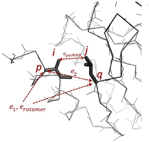
ABACUS energy terms. Two backbone position indices (p and q) and two sidechain atom indices (i and j) are indicated. The $e_1$ and $e_2$ are functions of residue types, $e_{\mathrm{rotamer}}$ is a function of the rotamer state and $e_{\mathrm{packing}}$ depends on sidechain atom positions, which are determined from backbone positions and rotamer states. During sequence design, the backbone atoms are fixed, the total energy is optimized with respect to the residue types and rotamer states

2.1.2 The single residue energy term that depends on the residue type

In ABACUS2, this term measures the residue type preference given local structural features including the secondary structure (SS) type, the Ramachandran backbone φ and ψ torsional angles (RAMA) and the solvent accessibility index (SAI) (Xiong et al., 2014) or formally,

$$e_1\left(a_p=a||\mathit{backbone}\right)\equiv e_1\left(a||\mathit{S}{\mathit{S}}^p,\mathit{RAM}{\mathit{A}}^p,\mathit{S}{\mathit{AI}}^p\right)+e_{\mathit{ref}}\left(a\right|\mathit{S}{\mathit{S}}^p)$$

(6)

in which $\mathit{S}{\mathit{S}}^p$⁠, $\mathit{RAM}{\mathit{A}}^p$ and $\mathit{S}{\mathit{AI}}^p$ represent respective structure features of position p, which are all computed from the Cartesian coordinates of main chain atoms. The SAI values are calculated based on a refined pseudo sidechain model in ABACUS2. The SS type-dependent reference energies $e_{\mathit{ref}}\left(a|\mathit{S}{\mathit{S}}^p\right)$are determined at the final stage of the energy parameterization to reproduce the residue type frequencies in different SS types. They will be discussed later. Here we consider the derivation of the statistical energy $e_1\left(a|\mathit{S}{\mathit{S}}^p,\mathit{RAM}{\mathit{A}}^p,\mathit{S}{\mathit{AI}}^p\right)$⁠.

In the spirit of statistical energy functions (Miyazawa and Jernigan, 1985; Sippl, 1995; Zheng and Grigoryan, 2017) $e_1\left(a|\mathit{S}{\mathit{S}}^p,\mathit{RAM}{\mathit{A}}^p,\mathit{S}{\mathit{AI}}^p\right)=-\mathit{ln}P\left(a\right|\mathit{S}{\mathit{S}}^p,\mathit{RAM}{\mathit{A}}^p,\mathit{S}{\mathit{AI}}^p)$⁠, in which $P\left(a\right|\mathit{S}{\mathit{S}}^p,\mathit{RAM}{\mathit{A}}^p,\mathit{S}{\mathit{AI}}^p)$ refers to the probability of observing residue type a conditioned on a specific combination of the structural features. This probability is estimated from a set of training protein structures by considering the residue type distribution at those training protein backbone positions whose structural features are similar to those of the target position p.

In ABACUS1, the search for structurally similar positions in the training proteins has been carried out separately for every position in every design target. In ABACUS2, this search and the subsequent probability estimation have been pre-executed for a set of representative points in the structural feature space, generating once-and-for-all a set of pre-determined energy tables specifying the residue type-dependent energies in different regions of the structural feature space. When sequence design is carried out for an actual target backbone, the energy tables for the actual backbone positions are obtained by interpolation. More details are given in Supplementary Material.

2.1.3 The pairwise energy term that depends on the residue type pairing

This energy term measures the preferences of residue type pairing at two backbone positions that are sequentially or spatially close to each other. Unlike in many other statistical energy functions, where similar terms simply depend on certain inter-residue distances, in ABACUS, this energy term jointly depends on the local structural features (including the SS type and the SAI) of the two interacting sites, as well as on the relative geometries between the two sites. Namely,

$$\begin{array}{c}{e}_2\left(a_p,a_q|\mathit{backbone}\right)\equiv e_2\left(a_p,a_q|\mathit{S}{\mathit{S}}^p,\mathit{SA}{\mathit{I}}^p,\mathit{S}{\mathit{S}}^q,\mathit{SA}{\mathit{I}}^q,\mathit{SE}{\mathit{P}}^{\mathit{pq}},\mathit{RGEO}{\mathit{M}}^{\mathit{pq}}\right)\\ =w_2\left(\mathit{SE}{\mathit{P}}^{\mathit{seq}}\right)*\mathit{ln}\frac{P(a_p,a_q|\mathit{S}{\mathit{S}}^p, \mathit{SA}{\mathit{I}}^p,\mathit{S}{\mathit{S}}^q,\mathit{SA}{\mathit{I}}^q,\mathit{SE}{\mathit{P}}^{\mathit{pq}},\mathit{RGEO}{\mathit{M}}^{\mathit{pq}})}{P\left(a_p|\mathit{S}{\mathit{S}}^p,\mathit{SA}{\mathit{I}}^p\right)*P\left(a_q\right|\mathit{S}{\mathit{S}}^q,\mathit{SA}{\mathit{I}}^q)}\end{array}$$

(7)

in which p and q refer to two interacting backbone positions, SEP^pq refers to their sequence separation, and RGEOM^pq their relative geometry. The interactions for SEP^pq = 1, 2, 3 and 4 (local site pairs) have been treated separately as to be of different interaction types, while the interactions for SEP^pq > 4 (non-local site pairs) have been jointly considered to be of the same type. The scaling factor $w_2\left(\mathit{SE}{\mathit{P}}^{\mathit{seq}}\right)$ is used to compensate for the double counting of local interactions between different local site pair terms. Its value is 0.5 for SEP^pq$\hspace{0.5em}$≤ 4 and 1.0 for SEP^pq > 4.

As in the treatment of the single residue energy term, the joint structural feature space of backbone position pairs has been covered with representative points. For each point an energy table has been pre-constructed by retrieving structurally similar position pairs from the training proteins. During sequence design, the e₂ for actual site pairs in a design target will be calculated using interpolation. More details are given in Supplementary Material.

2.1.4 The single residue energy term that depends on the rotamer state

Sidechain conformations and inter-atomic packing are considered by using discrete rotamer states. The rotamer library used in ABACUS2 has been specifically refined to improve accuracy (see below). The backbone-dependent rotamer energy term $e_{\mathit{rotamer}}\left(x_{a_p=}{x}_a\right|\mathit{backbone})\equiv e_{\mathit{rotamer}}(x_a|{\mathit{\phi }}^p,{\mathit{\psi }}^p)$ for an actual backbone site p is obtained by interpolation using the pre-calculated energies at nearby representative φ–ψ points. More details are given in Supplementary Material.

2.1.5 The packing energy

The atomic packing energy in Equation (5)$e_{\mathit{packing}}\left(i,j|\mathit{backbone}\right)\equiv e_{\mathit{packing}}\left(r_{\mathit{ij}}\right)$ is determined using an empirical functional form. The parameters in this form have been derived from training proteins. This is different from ABACUS1 which uses an adjusted Lennard-Jones form with molecular mechanics parameters to describe packing. Based on the analysis of inter-atomic direct contacts as described in Supplementary Material, Equation (8) has been empirically defined to model the packing energy. It comprises a harmonic repulsive part and an inverted Gaussian attractive part to describe packing energies at inter-atomic distances below and above the optimum packing distance, respectively,

$$e_{\mathit{packing}}\left(r_{\mathit{ij}}\right)=\left\{\begin{array}{c}{\mathit{\lambda }}_{\mathit{ij}}*\left[{\frac{1}{2}k}_{\mathit{ij}}{\left(r_{\mathit{ij}}-{r_{\mathit{ij}}}^{\mathit{min}}\right)}^2-{e_{\mathit{packing}}}^{\mathit{min}}\right] \mathit{if} r_{\mathit{ij}}<{r_{\mathit{ij}}}^{\mathit{min}} \\ -{\mathit{\lambda }}_{\mathit{ij}}*{e_{\mathit{packing}}}^{\mathit{min}}*\hspace{0.17em}\text{exp}\hspace{0.17em}\left[-{\left(\frac{r_{\mathit{ij}}-{r_{\mathit{ij}}}^{\mathit{min}}}{d_{\mathit{ij}}}\right)}^2\right] \mathit{otherwise} \end{array}\right.$$

(8)

in which $r_{\mathit{ij}}$ is the actual distance between atoms i and j, and ${r_{\mathit{ij}}}^{\mathit{min}}\equiv {r_i}^{\mathit{min}}+{r_j}^{\mathit{min}}$ the corresponding optimum packing distance. The derivation of the atom type-specific half distances ${r_i}^{\mathit{min}}$ and ${r_j}^{\mathit{min}}$ is described in Supplementary Material. The interaction strength ${e_{\mathit{packing}}}^{\mathit{min}}$ depends on the polarity and aromaticity of both atoms i and j (Supplementary Table S5). The well-depth scaling parameter ${\mathit{\lambda }}_{\mathit{ij}}$⁠, the repulsive force constant $k_{\mathit{ij}}$⁠, the well-width parameter $d_{\mathit{ij}}$⁠, as well as the solvent accessibility-dependent weights ${w_{\mathit{packing}}}^{\mathit{pq}}$ in Equation (5) are described in Supplementary Material.

2.2 The refined pseudo sidechain model and rotamer library

2.2.1 Measuring solvent accessibility with a refined pseudo sidechain model

The structural feature SAI has been used to quantify the solvent accessibility of individual amino acid positions without specifying the types and conformations of sidechains. It has been derived using a pseudo sidechain model (Marshall and Mayo, 2001; Zhang et al., 2004) in which pseudo sidechains of the same type and the same internal geometry are ‘installed’ at all backbone sites. In ABACUS2, a refined pseudo sidechain model has been used to compute SAI, so that the mutual information between the calculated SAI and the residue type in native proteins is maximized. The mutual information has been calculated as

$$\mathit{MI}\left(N_{c_{\mathit{sa}}}\right)=\sum _{a=1}^{20}\sum _{c_{\mathit{sa}}=1}^{N_{c_{\mathit{sa}}\mathit{ }}}P\left(a,c_{\mathit{sa}}\right){\mathit{log}}_2\frac{P\left(a,c_{\mathit{sa}}\right)}{P\left(a\right)p\left(c_{\mathit{sa}}\right)},$$

(9)

in which a is the residue type,$\mathit{ }{N}_{c_{\mathit{sa}}}$ the number of solvent accessible categories, c_sa the solvent accessibility category defined based on the calculated SAI and $P\left(a,c_{\mathit{sa}}\right), P\left(a\right) \mathit{and} P\left(c_{\mathit{sa}}\right)$ the respective joint or marginal probabilities. More details are given in Supplementary Material. The data in Table 1 show that SAIs computed with the new model have larger MI with residue type than previous methods.

Table 1.

Mutual information between the amino acid type and the solvent accessibility category determined by using different methods to measure the solvent accessibility of backbone positions in native proteins^a

Method	Number of solvent accessibility categories (⁠$N_{c_{\mathrm{sa}}}$⁠)
	2	3	4	5	6
Relative SASAb	0.136	0.159	0.170	0.176	0.180
Number of Cβ neighborsc	0.103	0.124	0.135	0.139	0.142
Pseudo sidechain, MEAd	0.129	0.151	0.167	0.176	0.181
Pseudo sidechain, PSDe	0.146	0.172	0.189	0.198	0.201

Note: Categorizations are based on dividing the respective measures into bins of even width. MEA, mean sidechain; PSD, pseudo sidechain.

a

A subset of TRN7258 containing 3000 native protein structures has been used.

b

Solvent accessibility is measured with the relative solvent accessible surface areas (SASA) of individual residues in native protein structures with complete sidechains.

c

Solvent accessibility is measured with the number of neighboring residues determined with an inter-C_β distance cutoff of 8 Å.

d

This pseudo sidechain model has been developed by Marshall and Mayo and used in ABACUS1.

e

This is the final model used in ABACUS2.

2.2.2 The refined rotamer library

In ABACUS1, a previously defined rotamer library (Ota et al., 2001) was used to consider discretely variable dihedral angles with fixed bond lengths and bond angles for a given sidechain type. In ABACUS2, a new rotamer library has been defined on the basis of not the internal coordinates but the Cartesian coordinates of sidechain atoms in a local coordinate frame determined by the backbone atom positions. Sidechain conformers in this new library have been taken from native protein structures. By using a Monte Carlo protocol similar to the one used to choose representative backbone position pairs, the conformers to include in the library have been optimally selected so that sidechain conformers in native proteins can be approximated by rotamers with the smallest overall RMSD. In addition, the number of rotamers for each residue type has been chosen to balance accuracy with efficiency.

2.3 Protein structure sets for training and for testing

They are given in Supplementary Material.

2.4 Sidechain conformation optimization and amino acid sequence design

2.4.1 Sidechain optimization

Sidechain repacking have been carried out using the Monte Carlo protocol described in Supplementary Material. The energy function optimized during sidechain repacking included the same sidechain-conformation-dependent rotamer energies and atomic packing energies as those considered in sequence design. One minor point is that the current ABACUS2 does not support the design of sequences containing disulfide bonds. In sidechain repacking, for cysteine sidechain pairs forming disulfide bonds, simple harmonic energies depending on the disulfide bond geometries (bond lengths, bond angles and torsional angles, see Supplementary Material) have been added. The sidechain repacking results for proteins in the TRN200 training set have been used to direct the optimization of the parameters in the rotamer and the packing energies [Equation (8) in main text and Equations (S8–S14) in Supplementary Material]. The objective has been to achieve the smallest RMSD from the native sidechain structures. The optimization process has been started with an initial set of intuitively selected parameters, followed by iterative manual adjustments of the parameters. In each iteration, a series of repacking calculations is carried with only one or two parameters systematically varied around their current values. In the next iteration, these parameters are updated with newer values that led to smaller RMSD and other parameters are varied systematically. Around the final set of parameters, extensive trial variations have been tested and the RMSD could not be further reduced. The optimized parameters have been used in subsequent side repacking tests and sequence design tests on a different set of test proteins.

2.4.2 Amino acid sequence design

In Figure 2, a flowchart of the Monte Carlo simulated annealing optimization-based protocol used in ABACUS2 to design amino acid sequences is given. More details are given in Supplementary Material. The sequence design results for proteins in the TRN40 training set (Supplementary Table S6) have been used to drive the optimization of the weightings of the packing term, including the secondary structure type-dependent reference energies, i.e. $e_{\mathit{ref}}\left(a\right|\mathit{S}{\mathit{S}}^p)$ in Equation (6), and the parameters in Equation (S14) in Supplementary Material, according to which the SAI-dependent packing weights ${w_{\mathit{packing}}}^{\mathit{pq}}$ in Equation (5) are determined. The parameters determining the packing weights have been optimized first, with all the reference energies set to zero. The objectives to minimize are the differences between the designed proteins and the native ones in their total numbers of atoms in the core, the intermediate and the surface regions, respectively. A grid search in the space of the four parameters has been carried out to find a set of optimum values. Then, all other parameters fixed, the residue type-specific reference energies have been iteratively adjusted so that all the training proteins considered together, the native occurrence rates of different residue types in different types of SS elements can be approximately reproduced by the redesigned proteins. The resulting reference energies are given in Supplementary Table S7.

Fig. 2.

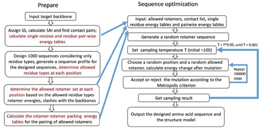
Flowchart of the sequence design process. The left side shows the prepare phase, while the right side shows sequence optimization via Monte Carlo simulated annealing

2.5 Preliminary experimental tests of sequences designed by ABACUS2

Preliminary experimental characterization of proteins designed using ABACUS2 have been carried out using nuclear magnetic resonance ¹H-¹⁵N heteronuclear single quantum coherence (HSQC) spectroscopy (Bodenhausen and Ruben, 1980) and circular dichroism (CD) (Adler et al., 1973). Three native backbone structures taken from PDB, 1ubq, 1r26 and 2qsb, have been considered as target backbones. Among them, 1ubq and 1r26 are of the α + β fold class, and 2qsb is a helix bundle (see Supplementary Fig. S6). Details of the experimental processes are given in the Supplementary Material.

3 Results and discussions

3.1 Mutual information between computed SAI and native residue type

In Table 1, the mutual information determined for the PSD pseudo sidechain model used in ABACUS2 is compared with the pseudo sidechain model used in ABACUS1, and with two other approaches from the literature, one considering the number of neighboring residues determined from C_β positions, and the other considering the relative solvent accessible surface areas of residues in all-atom protein structures. Compared with the other methods, the current method consistently leads to larger mutual information, irrespective of the choice of the number of solvent accessibility categories.

3.2 Errors of estimating the statistical energies through interpolation

3.2.1 The single residue energy term

To assess if the chosen set of representative points in the space of the single site structural features can cover that space with sufficiently high density and if the errors contained in the energy values estimated by interpolation are acceptably small, the single residue energy of each backbone position in the test proteins has been estimated by both the interpolation approach and a direct approach, in which the actual target position has been directly used as query to search for structurally similar positions in the training proteins to obtain an estimation of the single residue energy. The results are compared in Figure 3. When the energy of an actual backbone position is approximated using the pre-calculated energy of the single closest representative point, the RMS error is only 0.17 (Fig. 3a). If the interpolation scheme described in Supplementary Material is used, the RMS error is further reduced to 0.10 (Fig. 3b). The magnitudes of these errors are only ca. 1∼3% of the overall variable range of this energy term, which is between 0 and 6.

Fig. 3.

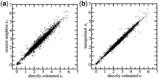
The single residue energies estimated by using representative points in the structural feature space compared with those estimated by direct search. (a) Estimations using the single nearest representative points. (b) Estimations using interpolation between multiple nearest representative points. Backbone positions are from proteins in the TRN40 set

3.2.2 The residue pairwise energy term

Given the optimized sets of representative backbone site pairs, the interpolation approach to estimate the residue pairwise energies introduces only small errors in comparison with the direct estimation approach, in which each actual target position pair is used as query to retrieve from the training proteins structurally similar backbone position pairs to estimate the residue pairwise energies. In Figure 4, the residue pair energies calculated using the interpolation approach and the direct estimation approach are compared. When the energy is approximated by the pre-calculated energy of the single most similar representative position pair, the RMS error is 0.19 (Fig. 4a). If the energy is calculated using the interpolation scheme in the Supplementary Material, the RMS error is reduced to 0.15 (Fig. 4b). These RMS errors are only 3∼4% in comparison with the variation range of this energy term, which is between −3 and 2.

Fig. 4.

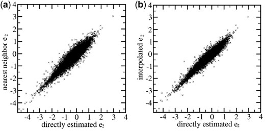
The residue pair energies estimated by using representative points in the structural feature space compared with those estimated by direct search. (a) Estimations using the single nearest representative points. (b) Estimations using interpolation between multiple nearest representative points. Backbone positions are from proteins in the TRN40 set

3.3 Quality of the rotamer library and the accuracy of sidechain repacking

3.3.1 Atomic RMSDs of representing sidechain conformations by rotamers

The quality of different rotamer libraries to represent sidechain atomic positions has been compared by assigning native sidechain conformations to their respective closest rotamer states, and determining the RMSDs between the actual and the rotamer atomic positions. Compared with the rotamer library used in ABACUS1, the new library in ABACUS2 can represent sidechain atom positions in native proteins with much smaller atomic RMSDs using approximately the same number of rotamers (Table 2), probably because in the new library, internal coordinate other than the torsional angles, especially the bond angles have been allowed to vary between the different rotamer states of the same residue type.

Table 2.

The numbers of rotamers (⁠$N_{\mathrm{rot}}$⁠) for different residue types in ABACUS1 and ABACUS2, and the RMSDs of atomic positions (in Å) after replacing native sidechain conformations with those of the closest rotamers

Residue type	ABACUS1		ABACUS2
	$N_{\mathrm{rot}}$	RMSD	$N_{\mathrm{rot}}$	RMSD
ALA	1	0.0867	1	0.0458
CYS	9	0.1748	10	0.1324
ASP	24	0.333	20	0.2447
GLU	21	0.576	40	0.3974
PHE	36	0.4318	40	0.2603
GLY	1	0	1	0
HIS	24	0.4247	40	0.2983
ILE	15	0.2675	15	0.2209
LYS	38	0.6287	40	0.5106
LEU	15	0.4804	15	0.2259
MET	19	0.5643	50	0.3472
ASN	36	0.3685	30	0.2681
PRO	6	0.2911	6	0.1
GLN	24	0.6131	50	0.4228
ARG	45	0.8884	60	0.6876
SER	27	0.1507	6	0.1346
THR	27	0.1683	6	0.1434
VAL	9	0.1713	6	0.1357
TRP	72	0.5057	80	0.3323
TYR	72	0.4911	60	0.2702
Overall	521	0.381	576	0.259

Note: The RMSDs have been obtained on protein structures in the TRN7258 set. The overall results are highlighted in bold.

3.3.2 Results of the sidechain repacking tests

The accuracy of sidechain repacking has been measured by the RMSD of the predicted sidechain atom positions with respect to the X-ray structure, and by the proportion of residues with correctly predicted (the predicted values being within 40° of the corresponding actual values) χ₁ torsional angles or both χ₁ and χ₂ angles. Table 3 shows that ABACUS2 leads to notably reduced overall RMSD in comparison with ABACUS1, a combined effect of the refined rotamer library and the new functional forms and parameters for the backbone-dependent rotamer energy and the packing energy. When compared with other programs, including SCWRL4 (Krivov et al., 2009) and the Rosetta program with different rotamer sets (Leaver-Fay et al., 2011), ABACUS2 gives the smallest overall RMSD. Table 3 also includes RMSD results for sidechains in different solvent accessibility classes. While the results of all models obey the trend of showing decreasing accuracy (or increasing RMSD) for positions with increasing solvent exposure, ABACUS2 seems to give the smallest RMSD within each solvent accessibility class. Especially for the core and the intermediate classes, the results of ABACUS2 are notably better.

Table 3.

The atomic RMSD (in Å) of repacked sidechains with respect to native sidechains

Method	RMSD for regions of different solvent accessibility
	Core	Intermediate	Surface	All
ABACUS1	1.017	1.526	1.999	1.633
ABACUS2	0.554	1.148	1.804	1.353
SCWRL4	0.737	1.378	1.858	1.476
Rosetta default	0.850	1.422	1.910	1.531
Rosetta ex1	0.753	1.361	1.883	1.484
Rosetta ex2	0.672	1.338	1.870	1.461
Rosetta ex3	0.654	1.331	1.890	1.467
Rosetta ex4	0.673	1.326	1.891	1.467

Note: Results from different methods are given and the results of ABACUS2 are highlighted in bold. The RMSDs have been calculated on the TST40 set of native structures. The rows Rosetta default to Rosetta ex4 correspond to results obtained using rotamer sets of increasing sizes and finer conformation resolutions.

In Table 4 and Supplementary Tables S8 and S9, the residue type-specific RMSDs and ratios of residues with correctly predicted sidechain torsional angles from sidechain repacking carried out with different models are compared. For most residue types, ABACUS2 gives similar or lower RMSDs as well as higher ratios of correctly predicted torsional angles than SCWRL4 or Rosetta. The residue types for which ABACUS2 gives notably better results are the aromatic ones, including Trp, Phe and Tyr. Controlling calculations (data not shown) suggested that to a large extent, the improvement could be attributed to that orientation-dependence have been used to treat packing involving aromatic rings (see Supplementary Material).

Table 4.

The same as Table 3, only that is, results for different residue types are listed separately

	ABACUS1	ABACUS2	SCWRL4	Rosetta default	Rosetta ex1	Rosetta ex2	Rosetta ex3	Rosetta ex4
CYS	0.712	0.446	0.561	0.542	0.559	0.477	0.619	0.546
ASP	1.323	0.977	1.105	1.155	1.147	1.153	1.144	1.129
GLU	2.071	1.697	1.67	1.724	1.722	1.687	1.716	1.74
PHE	1.22	0.792	0.988	1.127	1.034	1.074	1.042	1.047
HIS	1.995	1.957	1.734	1.936	1.815	1.833	1.858	1.873
ILE	0.711	0.531	0.645	0.698	0.645	0.631	0.62	0.612
LYS	2.174	1.958	1.986	1.971	2.001	1.929	1.993	1.977
LEU	0.905	0.745	0.886	0.861	0.802	0.75	0.753	0.765
MET	1.644	1.207	1.496	1.53	1.477	1.385	1.405	1.415
ASN	1.521	1.321	1.311	1.306	1.283	1.286	1.285	1.261
PRO	0.48	0.315	0.297	0.287	0.286	0.288	0.278	0.281
GLN	1.949	1.701	1.836	1.812	1.738	1.801	1.741	1.789
ARG	2.809	2.445	2.745	2.746	2.694	2.607	2.644	2.627
SER	0.926	0.828	0.9	0.871	0.845	0.849	0.86	0.864
THR	0.656	0.601	0.687	0.653	0.622	0.605	0.605	0.615
VAL	0.601	0.555	0.581	0.669	0.624	0.596	0.598	0.59
TRP	1.975	1.051	1.861	2.151	2.014	2.059	1.92	1.986
TYR	1.492	0.974	1.127	1.43	1.27	1.254	1.264	1.212

Note: The results in ABACUS2 are highlighted in bold.

3.4 Complete sequence redesign using ABACUS2

3.4.1 Native residue type recovery rates from the sequence redesign tests

The native residue type recovery rate refers to the proportion of sites that were occupied by corresponding native residue types in the redesigned sequences. We emphasize that throughout the training and parameterization processes of the ABACUS2 model, protein-specific or site-specific recovery of the native residue type has not been considered as a goal to be maximally achieved. Thus this measure can be considered as an appropriate indicator for the quality of the method, if we assume that the majority of native sequences should be sufficiently close to the optimum ones to stabilize the respective native backbones. For each target in the test set of proteins TST40 (Supplementary Table S6), five sequences have been designed using each method considering only the native backbone as input without any sequence restraints, the native recovery rates averaged over these sequences. In Table 5, the native residue type recovery rates of ABACUS1, ABACUS2 and RosettaDesign with fixed backbone are compared. Supplementary Figure S7 shows that for 32 out of 40 targets, ABACUS2 achieves increased recovery rates over ABACUS1. The overall improvement is substantial (from 32.7 to 37.7%, Table 5). The improvements mainly come from the residue choices at the buried (core) and the partially buried (intermediate) positions. This is consistent with the results of the sidechain repacking tests, which shows that ABACUS2 can reproduce the sidechain atomic positions of (partially) buried sidechains with much higher accuracy than the ABACUS1. For the solvent-exposed (surface) backbone sites, ABACUS2 still performs slightly better than ABACUS1, suggesting that while speeding up the computation significantly, the interpolation approach to calculate statistical energies in ABACUS2 does not lead to deterioration of the final design results. Compared with the RosettaDesign fixed backbone results, the overall native residue type recovery rate of ABACUS2 is moderately larger (37.7 versus 35.9%) for the given set of test proteins. The main difference comes from the surface positions, for which both the ABACUS1 and ABACUS2 models are notably more likely to choose the respective native residue types than fixed-backbone RosettaDesign. For the partially exposed positions, only the ABACUS2 model can outperform fixed-backbone RosettaDesign. For the core positions, the ABACUS2 and fixed-backbone RosettaDesign perform comparably.

Table 5.

The rates of recovering the native residue type in fixed-backbone sequence design^a

Method	Native recovering rate for regions of different solvent accessibility
	Core	Intermediate	Surface	All
ABACUS 1	0.501	0.274	0.263	0.327
Rosetta	0.606	0.323	0.237	0.359
ABACUS2	0.590	0.342	0.274	0.377

a

The results have been obtained on backbone structures contained in the TST40 set of native proteins.

Note: The results in ABACUS2 are highlighted in bold.

3.4.2 Experimental characterization of sequences designed by ABACUS2

Five of the nine designed proteins (Supplementary Table S10) express well in Escherichia coli using protocols described in Supplementary Material. They are all the three designed proteins using 1ubq as target, the 1r26_1 designed for target 1r26 and the 2qsb_2 designed for target 2qsb. There was no detectable protein expression for the remaining designed proteins, probably because of the lack of optimization of the protein expression conditions. The HSQC spectra of the well-expressed proteins signal well-folded structures (Fig. 5) (Kwan et al., 2011). Temperature-dependent CD have been carried out on the α + β type proteins 1ubq_1 and 1r26_1, results shown in Supplementary Figure S8. Similar to other de novo designed proteins, the CD spectrum does not show much change with increasing temperature, indicating the high thermo-stability of secondary structure elements (Adler et al., 1973). The results in Figure 5 and Supplementary Figure S8 indicate that just as proteins designed using ABACUS1, the proteins designed by ABACUS2 for native backbone targets can be well-folded. As it has already been shown that the experimentally solved structures of proteins designed using ABACUS1 agree well with respective target structures (Xiong et al., 2014; Zhou et al., 2016) and the accuracy of ABACUS2 is improved over ABACUS1 according to the native residue type recovery rate, we do not extend the experimental work into solving the structures of these designed proteins.

Fig. 5.

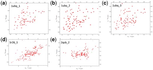
¹H-¹⁵N-HSQC spectra of designed proteins. (a–c) Spectra of three sequences designed for the target backbone 1ubq. (d) Spectrum for a sequence designed for the target backbone 1r26. (e) Spectrum for a sequence designed for the target 2qsb

3.5 Increase in speed and a web server

The computational cost of ABACUS2 is reduced by more than 90% relative to ABACUS1 (see Supplementary Fig. S9). Typical cost of sequence design applying the current un-optimized code for a protein of ca. 100 residue is about 10–15 min using a single core of the CPU of a common personal computer. Future parallelization and optimization of the code should be able to reduce the wall-clock time by another one or two order of magnitude.

A web server is provided for the online use of ABACUS2. The user interface is simple and straightforward. The target backbone structure is uploaded in PDB format and the results including the sequences, structures and energy components of the designed proteins are returned in a downloadable compressed archive file. The amino acid residue types contained in the input PDB file are ignored in unrestrained sequence design, which is the default. Alternatively, the designed sequences can be restrained by user-specified allowed amino acid residue types at a list of positions. In addition, as the optimized sequences for different free Monte Carlo runs are usually highly similar to each other, we have implemented options to enforce user-specified restraints on the extent of sequence divergence between the designed sequences, or between the designed sequence and the reference sequence provided in the input PDB data. One can also use the web server as an analytic tool, namely, to evaluate the sequence energy of a protein structure without redesigning the sequence. The result is broken into contributions of different interaction types (single position, position pair, rotamer, etc.) associated with individual backbone positions.

We would like to emphasize to users of the server that the ABACUS method only addresses the problem of sequence design for given backbones, one of the essential sub problems of the overall protein design problem (Liu and Chen, 2016). To apply ABACUS, a presumably designable target backbone, either taken from an existing protein structure or artificially constructed using other approaches, is needed. When ABACUS is applied to existing structures, it has been found that the designed sequences that fold into expected structures are likely to have much higher stability than their native counterparts: for examples, the denaturing guanidine concentration of the designed protein Dv_1ubq (PDB ID 2MLB) is around 7M versus 4M of the corresponding native protein (Xiong et al., 2014); the melting temperature of the designed protein E_1r26 (PDB ID 2NBS) (Zhou et al., 2016) is 118°C measured by differential scanning calorimetry versus the 54°C of the corresponding native protein (HMJ Minjie Han et al., unpublished data). Thus besides enabling sequence design for de novo backbones, the program can also be applied to improve existing functional proteins, for example, by fixing the residue types at functionally important interfaces while redesigning the rest of the protein to gain improved stability. It may also be applied to evaluate sequence-structure compatibility, such as the compatibility between fragments of functional sequence (for example, an immunogenic amino acid sequence segment) with a backbone segment embedded in an overall protein structure.

4 Conclusions

As an automated sequence design method that relies mainly on statistical energy terms, ABACUS complements most other current protein design programs which employed physics-based interactions as major components of their energy functions. One unique feature of ABACUS is that various structural features are considered jointly in single statistical energy terms. In ABACUS2, this has been realized in a computationally much more efficient way, which employs pre-determined representative points in respective high-dimensional structural feature spaces. A number of components in ABACUS1 has also been re-optimized. As a result, the accuracy as measured by the native residue type recovery rate has also been improved from 32.7% of ABACUS1 to 37.7% of ABACUS2. Interestingly, the ABACUS2 model seems to be able to achieve higher native sequence recovery rate for surface positions than those mainly-physics-based methods. The improved computational efficiency of ABACUS2 allows it to be used in a web server. In addition, it may also be applied to construct sequence design protocols that consider a large number of alternative backbone structures, or to predict sequence profiles from structures for a large structural database.

Funding

This work was supported by the National Natural Science Foundation of China [U1732156 and 31470717 to Q.C., 21773220 and 31570719 to H.L.]; and Youth Innovation Promotion Association Chinese Academy of Sciences [2017494 to Q.C.].

Conflict of Interest: none declared.