


Abstract
Quantitative structure–activity relationship (QSAR) modelling is currently used in multiple fields to relate structural properties of compounds to their biological activities. This technique is also used for drug design purposes with the aim of predicting parameters that determine drug behaviour. To this end, a sophisticated process, involving various analytical steps concatenated in series, is employed to identify and fine-tune the optimal set of predictors from a large dataset of molecular descriptors (MDs). The search of the optimal model requires to optimize multiple objectives at the same time, as the aim is to obtain the minimal set of features that maximizes the goodness of fit and the applicability domain (AD). Hence, a multi-objective optimization strategy, improving multiple parameters in parallel, can be applied. Here we propose a new multi-niche multi-objective genetic algorithm that simultaneously enables stable feature selection as well as obtaining robust and validated regression models with maximized AD. We benchmarked our method on two simulated datasets. Moreover, we analyzed an aquatic acute toxicity dataset and compared the performances of single- and multi-objective fitness functions on different regression models. Our results show that our multi-objective algorithm is a valid alternative to classical QSAR modelling strategy, for continuous response values, since it automatically finds the model with the best compromise between statistical robustness, predictive performance, widest AD, and the smallest number of MDs.
The python implementation of MaNGA is available at https://github.com/Greco-Lab/MaNGA.
Supplementary data are available at Bioinformatics online.
1 Introduction
Quantitative structure–activity relationship (QSAR) methods have been widely applied in different fields such as toxicity prediction and drug design (Cherkasov et al., 2014). QSAR models link the numerical description of molecular structures, the molecular descriptors (MDs), to their known physical–chemical properties and biological activities (Cherkasov et al., 2014; Todeschini and Consonni, 2009). Despite continuous methodological developments in the QSAR field, obtaining accurate, reliable and stable models can still be challenging. A large number of easily computable descriptors, such as topological indices, two-dimensional (2D) and three-dimensional (3D) fingerprints are of utmost use to describe chemical structures (Todeschini and Consonni, 2009; Tropsha, 2010). However, selecting an optimal combination of predictive MDs in QSAR modelling is analytically difficult (Goodarzi et al., 2012). A comprehensive search of the best subset of features is computationally expensive, since as many as possible subsets of features for a dataset with N descriptors can be considered. Different methods for feature selection have been used in QSAR studies, such as multi-variate adaptive regression splines and lasso (Eklund et al., 2012), random forest importance selection (Svetnik et al., 2003), univariate methods (Liu, 2004), backward elimination and forward selection (Yasri and Hartsough, 2001). Particular attention has been given to optimization search strategies such genetic algorithms (Leardi, 2001). QSAR models should ideally contain the smallest set of MDs with best goodness of fit. Indeed, considering the Topliss and Costello rule (Topliss, 1972), the number of MDs should be smaller than 1/5 of the training set compounds. Multi-objective optimization has, therefore, been applied to identify the smallest set of MDs with the highest predictive ability. For example, Nicolotti et al. (2002) proposed two multi-objective methods that use genetic programming to provide an adequate compromise between the number of model descriptors and accuracy. Soto et al. (2009) developed a two-step feature selection using a multi-objective genetic algorithm that first performs a preliminary screening of the possible optimal solutions and, in a second step, enables model refinements. Recently Barycki et al. suggested a multi-objective genetic algorithm as a feature selection strategy for the development of ionic liquids’ quantitative toxicity–toxicity relationship models, where the same set of features was evaluated against multiple endpoints (Barycki et al., 2018). Another important challenge related to the modelling of high-dimensional data is the stability of the selected features, i.e. how stable the selected features are with respect to variations in the training set (Kalousis et al., 2007). Model stability may become of particular concern when the number of features is much higher than the number of compounds (Fortino et al., 2014), as it is in QSAR datasets (Goodarzi et al., 2012). Stability is usually neglected in traditional QSAR applications, where a single endpoint is predicted. However, considering the role of QSAR in the context of safe by design, stability becomes important for obtaining more robust and reproducible models. Thus, stability should be reported along with the other validation metrics. Moreover, the criteria established by the Organization for Economic Co-operation and Development (OECD) (OECD, 2014) must be met to ensure the validity of QSAR models. Along with the criteria addressing the transparency as well as internal and external statistical validity (Chirico and Gramatica, 2012; Consonni et al., 2009,, 2010; Golbraikh and Tropsha, 2002; Shi et al., 2001), a QSAR model is only reliable and valid with a defined applicability domain (AD) (Gramatica, 2007). The AD is the theoretical extent of the structural and response spaces in which the model is applicable to make reliable predictions for compounds with no experimental data. In brief, a good QSAR model should exhibit the best compromise between the number of MDs, predictive performance and the widest AD. To date, QSAR modelling has been traditionally carried out by following certain sequential steps: (i) data preprocessing (preparation of the modelable dataset and training/test set splitting), (ii) feature selection and modelling based on the optimization of individual parameters considered separately (e.g. R2), (iii) internal and external validation of the models and (iv) AD definition (Cherkasov et al., 2014; Gramatica, 2007,, 2013; Gramatica et al., 2013; Roy, 2007; Tropsha, 2010; Tropsha and Golbraikh, 2007). In general, these steps are followed iteratively until the best model is identified. Also, each step is usually considered separately, not allowing a holistic evaluation.
In a multi-objective optimization problem, multiple objective functions are involved. More formally, a multi-objective optimization problem can be formulated as follows: , where is the number of objective functions, while X is the set of feasible decision vectors, that is defined by the constraint functions (Konak et al., 2006). In many cases, multiple objectives under consideration conflict with each other, thus, the optimization with respect to a single objective can lead to unacceptable results with respect to the others. A good compromise is to identify a set of solutions that satisfy the objective at different levels and are not dominated by other solutions, meaning that they cannot be improved with respect to any objective without worsening at least one other objective (Konak et al., 2006). The set of all feasible non-dominated solutions is called Pareto optimal set, and their corresponding objective values are called Pareto front. Different multi-objective optimization approaches have been proposed with particular emphasis on evolutionary algorithms such as genetic algorithms (Konak et al., 2006). Here, we propose a new multi-objective strategy based on genetic algorithms that simultaneously enables stable feature selection as well as robust and validated regression models with an optimal AD.
2 Materials and methods
2.1 Multi-niches multi-objective genetic algorithm
Single- and multi-objective genetic algorithms were applied for feature selection in high-dimensional QSAR modelling. A multi-niche multi-objective genetic algorithm (MaNGA) (Fig. 1), was implemented to compare the behaviour of 15 different objective functions (Table 1) and to select the most stable solutions in terms of feature robustness. The multi-objective non-dominated sorting genetic algorithm II (NSGA-II) (Deb et al., 2002) was implemented in python with the distributed evolutionary algorithms in python (DEAP) computational framework (Fortin et al., 2012). The pseudocode of the MaNGA algorithm is available as Supplementary File S1. The NSGA-II algorithm was selected since it guarantees less computational complexity compared to other evolutionary algorithms and uses elitism to prevent the loss of good solutions among different iterations. In the proposed method, the individual solutions are binary chromosomes of length equal to the number of MDs in the dataset. A one (or zero) in the ith position indicates that the ith feature is (or is not) selected to be in the solution. Niching methods segment the genetic algorithm population containing n individuals, into k disjoint sets Ni with , called niches, such as whenever . These methods lead to a better cover of the searching region and of the local optima. MaNGA is implemented with a multi-niche schema with 20 different niches independently evolving their own populations by means of crossover and mutation. The niches interact between them by a genetic operator called migration that swap the top best 25% element of their populations, selected with the Pareto strategy. The interaction between the niches was implemented by using a Queue structure. Every niche contains a population of 500 individuals, with a mutation rate of 5% evolving for 500 generations. The best parameters setting was determined prior to running the genetic algorithm by preliminary analyses.
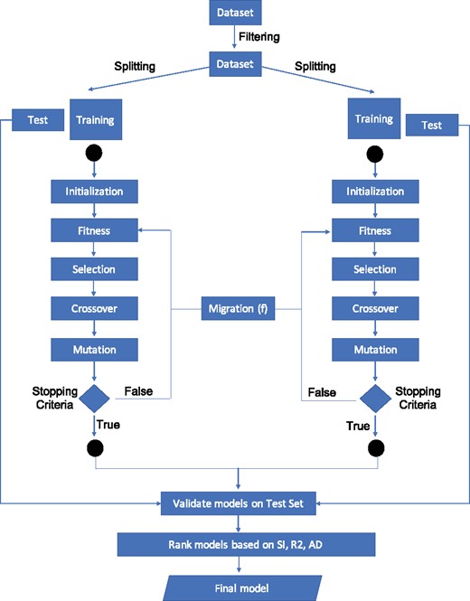
Multi-niches multi-objective genetic algorithm methodology: a multi-objective multi-niches genetic algorithm that is able to identify smaller and stable sets of molecular descriptors that better predict activity with an optimal applicability domain (AD)
Objective functions and internal and external evaluation metrics
| Original dataset | ||||||||||||||||||
|---|---|---|---|---|---|---|---|---|---|---|---|---|---|---|---|---|---|---|
| Training set | Test dataset | |||||||||||||||||
| Objective functions combination for feature selection | Internal validation | External validation | ||||||||||||||||
| Min/Max | Base function | I | II | III | IV | V | VI | VII | VIII | IX | X | XI | XII | XIII | XIV | XV | ||
| ↑ | R 2 | x | x | x | x | x | x | x | x | >RMSEtr | RMSEte | |||||||
| ↓ | RMSE | x | x | x | x | x | x | x | x | >ADtr | ADte | |||||||
| ↑ | AD | x | x | x | x | x | x | x | x | >Q2 | CCCte | |||||||
| ↑ | Q 2 | x | x | x | x | x | x | x | x | > | ||||||||
| ↑ | x | x | x | x | x | x | x | x | > | |||||||||
| ↓ | NFeat | x | x | x | x | x | x | x | x | > | ||||||||
Note: The 15 single- and multi-objective functions implemented in this work are reported (marked with Roman number) as combination of 6 base functions: R2, RMSE, AD, Q2, and NFeat. The x symbol is used to specify which base functions compose the objective functions. Furthermore, the list of internal and external validation metrics is reported. The threshold for the metrics are the following: ADte = 100, CCCte > 0.85, , NFeat < 1/5 of the no. of training set samples. Arrows show if the objective functions have to be minimize or maximize.
2.2 Objective functions and evaluation criteria
MaNGA was applied to explore the feature space that optimizes the fitness functions (Table 1). In particular, the first class of fitness function called the R2, maximizes the R2, Q2 and . The second class of fitness function, defined as MSE minimizes the mean-squared error in cross-validation on the training set. The third class of objective function called NFeat is meant to minimize the number of MDs selected by the GA. The AD objective function aims at maximizing the AD of the models both on the training and test set samples. These objective functions were combined to create 15 single- and multi-objective functions in which performances in the MaNGA method were investigated. For every niche, 20% of the original dataset was set aside as the test set, and not used in the model selection phase, but only to externally validate the trained model. The remaining 80% of the dataset was used to perform feature selection, train and internally validate the model, by using a 5-fold cross-validation repeated three times (Table 1). In order to check the stability of the feature selection algorithm, for every niche, a different training/test sets split was generated. Different regression models were compared. In particular, linear regression model (Freedman, 2009), support vector regression (Basak et al., 2007) and k-nearest neighbours (kNN) for regression (Zhou and Li, 2005) were implemented. Once the multi-objective optimization and feature selection step was performed, a pool of pareto-front optimal solutions were identified as the first output of the MaNGA algorithm. Thus, predictive performances for these models were evaluated in terms of the up-to-date criteria for QSAR models. Independently from the objective function used in the optimization process, RMSEtr (Aptula et al., 2005), the coefficient of determination , the leave-more-out correlation coefficient , the and the ADtr were computed, on the training set as internal validation metrics, for every model. Furthermore, the RMSEte (Aptula et al., 2005), , ADte and the concordance correlation coefficient CCCte were computed as external validation metrics on the test set. The detailed description of the evaluation metrics is reported in Table 2.
Evaluation metrics formulas and their accepted thresholds
| Metric | Min/max | Threshold | References |
|---|---|---|---|
| Min | Aptula et al. (2005) | ||
| Max | Golbraikh and Tropsha (2002) | ||
| Max | Golbraikh and Tropsha (2002) | ||
| Max | Chirico and Gramatica (2012), Shi et al. (2001) | ||
| Max | Chirico and Gramatica (2012), Schüürmann et al. (2008) | ||
| Max | Chirico and Gramatica (2012), Consonni et al. (2009, 2010) | ||
| Max | CCC > 0.85 | Chirico and Gramatica (2012) |
Note: Q2, and are computed with cross-validation strategies.
2.3 Number of features
An objective function minimizing the number of features to be included in each solution was introduced (Table 1). This objective function is optimized under the constraint that the MDs in the solutions do not exceed of the number of compounds in the training set. Solutions that do not satisfy this requirement were heavily penalized during the optimization process by assigning them a high fitness value. However, the maximum number of MDs in the solutions is a parameter of the algorithm that the user can change arbitrarily. Moreover, in order to easily converge to solutions satisfying the requirement, the initial binary population in every niche was generated with a probability of having value ‘0’ equal to 0.99 and value ‘1’ equal to 0.01.
2.4 Applicability domain
The AD was defined by means of the Williams plot based on standardized residuals and leverage values. The Williams plot helps identifying the response outliers as the ones following outside the 3σ range of the normally distributed standardized residuals that covers 99% of the samples. The leverage value (h) measures the distance from the centroid of the modelled space. A warning leverage, referred to as the critical hat value , is set at , where p is the number of variables appearing in the model and n is the number of samples in the training set. Thus, a compound was considered influential and identified as a high-leverage compound if . In a Williams plot (Gramatica, 2007), the leverage values were mapped against the standardized residuals to define the structural and the response spaces visually. Finally, the AD was reported as the percentile coverage for the training (ADtr) and the test (ADte) set, respectively. Solutions with ADte less than 100% were heavily penalized during the optimization process by assigning them a negative fitness value.
2.5 Selection of the final model
Multi-objective optimization methods, give as a result a set of optimal solutions distributed over the Pareto front represent different compromises between the best values of the multiple objectives to be optimized. Indeed, at the end of the iterations, a pool of 200 solutions was obtained by selecting the first 10 ranked solutions from every niche. However, as per traditional QSAR, a subsequent step for the models prioritization was carried out. Hence, every solution was further validated on the test set. Among these solutions, the unique sets of selected features were identified and ranked based on their occurrence frequency over the pool of 200. The solutions were then filtered based on thresholds already established in the literature: (Golbraikh and Tropsha, 2002), (Golbraikh and Tropsha, 2002), (Golbraikh and Tropsha, 2002), (Chirico and Gramatica, 2012; Shi et al., 2001), and (Chirico and Gramatica, 2012; Consonni et al., 2009,, 2010; Schüärmann et al., 2008), CCCte > 0.85 (Chirico and Gramatica, 2012), ADte = 100. Only the solutions that satisfy these requirements were considered eligible. Finally, the most frequent solution surviving the filtering was selected as the best one.
2.6 Time-complexity analysis
The computational complexity of our method is bounded by the complexity of the NSGA-II algorithm, that is (Deb et al., 2002), where k is the number of objectives to be optimized (from 1 to 5 for our approach) and S is the population size (500 for our approach). The time complexity of the fitness functions are reduced to the time complexity of the regression methods for the evaluation of the subset of features. Let n be the number of compound in the training sample, and p the number of MDs, the time complexity for the multiple linear regression method is , the time complexity for the kernel support vector regression (SVR) a is and the time complexity for the kNN is O(np). Moreover, it has to be considered that the fitness function is computed in a repeated cross-validation strategy, with five folds and three repetitions. The computational complexity of each iteration of our MaNGA algorithm is given by , where R is the time complexity of the selected regression model. Finally, this has to be multiplied by the number of iterations (500 in our approach). Even though the method is computationally intensive compared with other FS methods (Guyon and Elisseeff, 2003), CPU time is not a crucial issue provided that the algorithm may be executed in a reasonable polynomial time and feature selection is not aimed to be applied in real time.
2.7 Simulated dataset
In order to test the effectiveness of the proposed method, two simulated datasets with different number of compounds and MDs were generated, where the association between the MDs and the response is known. First, the original matrix of descriptors from a subset of the drugs in the connectivity map database (CMap) (Lamb et al., 2006) was generated. For each drug, the respective 3D SDF file was downloaded from PubChem (Kim et al., 2016) and given in input to the DRAGON v. 7 software (Mauri et al., 2006) to compute 5325 MDs. The constant (>80%) and highly interrelated MDs (pairwise correlation among all pairs of descriptors [>95%]) were filtered, as suggested (Gramatica et al., 2013). Next, a population of true coefficients with only 10 relevant extracted from a normal distribution with mean 10 and standard deviation 2 were chosen, while the other non-relevant was set to zero. The relevant values were selected in order to obtain a full AD with all the drugs inside the AD range. Furthermore, the error term ϵ was defined as an independent random normal vector, with mean 0 and standard deviation of 0.1. The intercept value was set as , and the response variable y as was computed. Finally, the MDs correlated with the 10 relevant ones or correlated with the response y were removed. The thresholds used for the correlation filtering were −0.2 and 0.2. The first simulated dataset (called ) contains 77 drugs and 55 MDs. The second simulated dataset (called ) consists of 518 drugs and 115 MDs. Details on the simulated dataset are shown in Table 3. The two simulated datasets are available as Supplementary Files S2 and S3.
Simulated datasets
| Dataset | No. of comp. | MDs |
|---|---|---|
| 77 | 55 | |
| = 0.3 + 7.33 MD8 + 11.65 MD11 + 12.47 MD29 + 0.05 MD30 + 11.51 MD31 + 12.65 MD33 + 9.6 MD35 + 9.12 MD36 + 12.58 MD44 + 8.05S MD55 + ϵ | ||
| 518 | 115 | |
| = 0.3 + 10.09 MD10 − 9.50 MD15 + 8.72 MD17 + 9.79 MD22 + 12.70 MD25. + 7.75 MD26 + 14.01 MD27 + 8.32 MD55 + 12.95 MD64 + 8.62 MD65 + ϵ | ||
Note: The number of compounds and MDs and the generative models for the two synthetic datasets.
2.8 Fathead minnow acute toxicity dataset
A dataset was retrieved from the literature (He and Jurs, 2005) containing measured acute toxicity as 96-h pLC50 (in mmol/l unit) of 288 compounds to Pimephales promelas (fathead minnow). The 3D.SDF files were downloaded from PubChem (Kim et al., 2016) and used as input in the software DRAGON v.7 (Mauri et al., 2006) to obtain 5325 MDs. Unsupervised feature reduction was applied to filter the constant (>80%) and highly intercorrelated descriptors (pairwise correlation among all pairs of descriptors >95%) prior to training/test set splitting, and variable selection (Gramatica et al., 2013). After the preprocessing, 954 MDs were considered for further analysis. The list of compounds used in this study is available in Supplementary File S4.
3 Results and discussion
Here, we compared the performances of single- and multi-objective functions (Table 1), using linear and non-linear regressions, for QSAR modelling. We investigated the performance of our novel algorithm, MaNGA, on two simulated datasets. Furthermore, we present a case study on a fathead minnow acute toxicity dataset (hereafter referred to as log-mmol-acqua) (He and Jurs, 2005).
3.1 MaNGA algorithm selects relevant features in simulated datasets
In order to show the effectiveness of our proposed methodology, we tested the performances of the MaNGA algorithm on two simulated datasets with known optimal set of features. We compared different objective functions (comprising R2, RMSE, NFeat, AD and R2-RMSE-NFeat-AD) in combination with three regression models (linear, SVR and kNN). MaNGA was run with the following parameters: 500 individuals, 50 number of iterations, 5 niches. We selected the first 10 best solutions for every niche for a total of 50 solutions and investigated the set of features identified by the algorithm along with the internal and external validation metrics and the AD value. Our results proved that the MaNGA algorithm correctly preferred the selection of features belonging to the optimal solution, in both datasets (Supplementary Files S5 and S6).
When using the linear regression, the number of optimal MDs in the solutions is higher than the MDs in the solutions coming from SVM and kNN regressors (Tables 4 and 5). Moreover, the optimal solutions are not selected when solely minimizing the number of features. On the other hand, when performing the multi-objective optimization with both SVM and kNN regression, the best minimal set of features is included both in the solutions of the (all the features) and dataset (two out of three), respectively. With regards to the evaluation metrics, good predictive abilities were obtained by the models resulting from the optimization of the R2, MSE and multi-objective, while low predictive capacity is achieved by the models obtained by maximizing only the AD or minimizing the number of MDs.
Selected features, internal and external validation metrics and frequencies for the solutions of MaNGA run on the dataset
| ObjFun | Reg | NF | RMSEtr | RMSEte | ADtr | ADte | Q 2 | CCCte | Freq. | |||||
|---|---|---|---|---|---|---|---|---|---|---|---|---|---|---|
| R 2 | LR | 4/10 | 0.09 | 0.12 | 98.55 | 100 | 0.96 | 0.94 | 0.94 | 0.97 | 0.97 | 0.97 | 0.96 | 10.20 |
| RMSE | LR | 4/10 | 0.07 | 0.54 | 95.65 | 87.5 | 0.97 | 92.32 | 0.95 | 9.95 | 0.95 | 0.95 | 0.06 | 30.00 |
| AD | LR | 1/4 | 0.44 | 0.44 | 98.55 | 100 | 0.06 | −0.04 | −0.07 | 0.77 | 0.77 | −0.74 | 0.03 | 26.19 |
| NFeat | LR | 0/3 | 0.44 | 0.52 | 97.10 | 100 | 0.09 | 0.10 | −13.36 | −12.63 | −12.67 | −11.93 | 0.12 | 34.00 |
| R 2-RMSE-AD-NFeat | LR | 2/3 | 0.14 | 0.18 | 100 | 100 | 0.90 | 0.84 | 0.88 | 0.90 | 0.90 | 0.90 | 0.92 | 26.19 |
| R 2-RMSE-AD-NFeat | SVM | 3/3 | 0.06 | 0.11 | 98.55 | 100 | 0.98 | 0.98 | 0.95 | 0.97 | 0.97 | 0.96 | 0.96 | 24.00 |
| R 2-RMSE-AD-NFeat | kNN | 3/3 | 0.06 | 0.10 | 98.55 | 100 | 0.99 | 0.99 | 0.97 | 0.97 | 0.97 | 0.97 | 0.97 | 31.03 |
Note: MDs column show the MDs selected by the MaNGA algorithm. The best solutions are those with: (i) RMSEtr and values as close as possible to zero; (ii) ADtr and ADte as close as possible to 100; (iii) , Q2, and CCCte as close as possible to 1.
Selected features, internal and external validation metrics and frequencies for the solutions of MaNGA run on the SimD2 dataset
| ObjFun | Reg | NF | RMSEtr | RMSEte | ADtr | ADte | Q 2 | CCCte | Freq. | |||||
|---|---|---|---|---|---|---|---|---|---|---|---|---|---|---|
| R 2 | LR | 2/5 | 0.07 | 0.06 | 97.85 | 94.23 | 0.90 | 0.92 | 0.89 | 0.91 | 0.91 | 0.91 | 0.94 | 11.63 |
| RMSE | LR | 6/14 | 0.03 | 0.03 | 97.42 | 98.08 | 0.98 | 0.98 | 0.98 | 0.99 | 0.99 | 0.99 | 0.99 | 40.00 |
| AD | LR | 1/13 | 0.17 | 0.17 | 100 | 100 | 0.37 | 0.35 | 0.33 | 0.91 | 0.91 | 0.92 | 0.52 | 59.38 |
| NFeat | LR | 0/3 | 0.21 | 0.22 | 97.00 | 100 | 0.02 | 0.05 | 0.01 | 0.87 | 0.87 | 0.86 | 0.04 | 32.00 |
| R 2-RMSE-AD-NFeat | LR | 2/7 | 0.06 | 0.07 | 99.14 | 100 | 0.91 | 0.89 | 0.91 | 0.97 | 0.97 | 0.97 | 0.95 | 100 |
| R 2-RMSE-AD-NFeat | SVM | 2/3 | 0.05 | 0.05 | 99.79 | 100 | 0.95 | 0.95 | 0.94 | 0.88 | 0.88 | 0.87 | 0.97 | 50.00 |
| R 2-RMSE-AD-NFeat | kNN | 2/3 | 0.03 | 0.04 | 98.50 | 100 | 0.98 | 0.96 | 0.95 | 0.95 | 0.95 | 0.96 | 0.97 | 33.33 |
Note: MDs column show the MDs selected by the MaNGA algorithm. The best solutions are those with: (i) RMSEtr and values as close as possible to zero; (ii) ADtr and ADte as close as possible to 100; (iii) , Q2, and CCCte as close as possible to 1.
3.2 Multi-objective functions provide the best compromise between number of MDs, widest AD and goodness of fit
We applied the MaNGA algorithm to a fathead minnow acute toxicity dataset (He and Jurs, 2005) by using different single- and multi-objective functions, and three regression models. The AD and NFeat objective functions did not produce models that met all the validation requirements, indeed and Q2 were lower than 0.6 and CCCte was lower than 0.85 (Table 6). On the other hand, the models obtained by optimizing the R2, RMSE and R2-RMSE-AD-NFeat functions fulfilled all the validation criteria. Moreover, the number of features selected by the multi-objective function was lower than the one selected by the single-objective ones (Table 6). Furthermore, the AD coverages of the multi-objective function were slightly higher than those obtained with the single-objective ones (Table 6). This was particularly clear when investigating the scatterplot of the observed versus predicted values and the Williams plot (Fig. 2). Indeed, when MaNGA was run by only optimizing the AD values, none of the training or test set samples fell outside the AD (Fig. 2B), but the predictive performances of the model were quite low, with poor concordance between the predicted and experimental data (Fig. 2A). Thus, the model did not fulfill the criteria regarding the goodness of fit and the internal and external validation requirements ( for LR and SVR models, and and CCCte < 0.85 for LR, SVR and kNN models). When the optimization was carried out in terms of the number of selected MDs, the model contained only three features (Table 6), but there was no high concordance between the predicted and experimental data (Fig. 2C), and AD was not satisfactory (Fig. 2D). Moreover, this model did not fulfil the criteria regarding the goodness of fit and the internal and external validation requirements ( for LR and SVR models and and for LR, SVR and kNN models, Table 6). On the other hand, when the optimization was performed by minimizing the MSE or maximizing the R2, the prediction capability of the model was better. Indeed Figure 2E and G shows a good concordance between the predicted and experimental data (), the solutions satisfied all the requested parameter of internal and external validation, but the AD values decreased to 94.21% on the training set when optimizing for the MSE (Fig. 2F, Table 6) and to 94.96% on the training set when optimizing for the R2 (Fig. 2H, Table 6). Moreover, the number of MDs in the models increased to 15 and 13 for MSE and R2, respectively (Table 6). The multi-objective optimization strategy allowed to meet as many requirements as possible with the same solution, particularly, when the optimization was performed by minimizing the number of features and the RMSE while maximizing the R2 and AD (Fig. 3). Moreover, using a non-linear model such as kNN (Fig. 3C and D) or SVR (Fig. 3E and F) significantly improved the goodness of fit of the model compared to the linear regression (Fig. 3A and B). The selected models are available in Supplementary File S7. The predicted values for the multi-objective function R2-AD-RMSE-NFeat for the linear, SVR and kNN models are reported in Supplementary Files S8–S10.
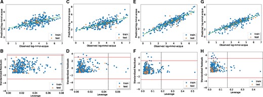
Comparison of the results obtained from the linear regression model with single-objective functions. The observed versus predicted log-mmol-acqua values (A) and the Williams plot representing the AD (B) of the linear model maximizing the AD. The observed versus predicted log-mmol-acqua values (C) and the Williams plot representing the AD (D) of the linear model minimizing the NFeat. The observed versus predicted log-mmol-acqua values (E) and the Williams plot representing the AD (F) of the linear model minimizing the MSE. The observed versus predicted log-mmol-acqua values (G) and the Williams plot representing the AD (H) of the linear model maximizing the R2
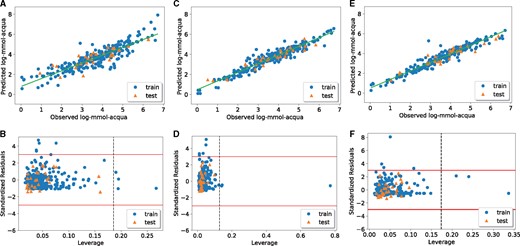
Comparison of the results obtained with multi-objective functions that maximize the R2, and AD while minimizing the number of features and MSE. The observed versus predicted log-mmol-acqua values (A) and the Williams plot representing the AD (B) of the linear model. The observed versus predicted log-mmol-acqua values (C) and the Williams plot representing the AD (D) of kNN model. The observed versus predicted log-mmol-acqua values (E) and the Williams plot representing the AD (F) of the linear model minimizing the MSE. The observed versus predicted log-mmol-acqua values (G) and the Williams plot representing the AD (H) of the SVR model
Multi-objective results for different training/test splits for each niche
| ObjFun | Reg | NF | RMSEtr | RMSEte | ADtr | ADte | Q 2 | CCCte | Freq. | |||||
|---|---|---|---|---|---|---|---|---|---|---|---|---|---|---|
| R 2 | LR | 13 | 0.59 | 0.53 | 94.98 | 100 | 0.78 | 0.85 | 0.75 | 0.68 | 0.68 | 0.7 | 0.85 | 13.64 |
| RMSE | LR | 15 | 0.53 | 0.63 | 94.21 | 100 | 0.82 | 0.74 | 0.79 | 0.61 | 0.61 | 0.6 | 0.88 | 33.33 |
| AD | LR | 6 | 1.00 | 0.91 | 100 | 100 | 0.42 | 0.48 | 0.38 | 0.74 | 0.73 | 0.76 | 0.56 | 33.33 |
| NFeat | LR | 3 | 0.93 | 0.83 | 97.30 | 100 | 0.49 | 0.59 | 0.46 | 0.74 | 0.74 | 0.73 | 0.63 | 28.38 |
| R 2-RMSE-AD-NFeat | LR | 5 | 0.62 | 0.63 | 95.75 | 100 | 0.78 | 0.83 | 0.76 | 0.88 | 0.88 | 0.86 | 0.86 | 12.82 |
| R 2-RMSE-AD-NFeat | SVM | 14 | 0.36 | 0.45 | 97.30 | 100 | 0.92 | 0.91 | 0.83 | 0.91 | 0.91 | 0.92 | 0.89 | 20.93 |
| R 2-RMSE-AD-NFeat | kNN | 10 | 0.39 | 0.44 | 96.91 | 100 | 0.91 | 0.89 | 0.81 | 0.86 | 0.86 | 0.88 | 0.88 | 22.22 |
Note: The table reports the results for the dataset log-mmol-acqua, for each objective function and for each regression model. Optimal solutions have R2 close to 1, FReq close to 100, RMSE close to 0, NF as small as possible and AD close to 100. Validation criteria fulfilled are in bold. The best solutions are those with: (i) RMSEtr and values as close as possible to zero; (ii) ADtr and ADte as close as possible to 100; (iii) , Q2, and CCCte as close as possible to 1.
3.3 Analysis of selected descriptors
Next, we analyzed the MDs selected by the MaNGA algorithm on the fathead minnow acute toxicity dataset by their occurrence frequency across the generated models. The most frequently selected MD was BLTD48. BLTD48 is the Verhaar Daphnia (48-h) base-line toxicity from MLOGP (mmol/l), a molecular property negatively relating to the Moriguchi hydrophobicity () (Moriguchi et al., 1992; Verhaar et al., 1992). BLTD48 showed a negative coefficient in the two linear regression models obtained with the MSE and R2 objective functions. The inverse relationship between the BLTD48 and MLOGP ultimately suggests that increasing hydrophobicity accounts for increasing toxicity. The second most frequently selected MD is another hydrophobicity term, the squared Ghose-Crippen octanol–water partition coefficient, ALOGP2 (Ghose et al., 1998). ALOGP2 showed a positive coefficient in the linear regression model when optimizing for the RMSE, thus, explaining increasing aquatic toxicity. Different octanol–water partition coefficients calculated based on different approaches, such as atomic contribution in the case of ALOGP and property-based methods in the case of MLOGP, have been reported elsewhere (Martin et al., 2015). Other MDs selected by more than one model are the Mor12s, nN, P_VSA_logP_3 and Ui. Mor12s is the signal-12 3D-MoRSE descriptor weighted by the intrinsic state (I-state). The I-state of an atom is the possible partitioning of the influence of non-σ electrons throughout the σ bonds within a molecule starting from the atom in consideration (Todeschini and Consonni, 2009). Hence, the less partitioning of the electron influence can be attributed to that the valence electrons are more prone to intermolecular interactions, which possibly result in toxicity. nN is a constitutional index counting the number of nitrogen atoms in a molecule also reported to be correlated to fathead minnow acute toxicity (Papa et al., 2005). P_VSA_logP_3 (P_VSA-like on LogP, bin 3) is a MD defined as the amount of van der Waals surface area (VSA) having a property in a certain range and is related to hydrophobicity (Labute, 2000). Finally, Ui is another molecular property descriptor representing the unsaturation index. The complete list of descriptors selected by MaNGA is available in Supplementary File S11.
3.4 Comparison with previous models
We compared our models for fathead minnow acute toxicity, with previously independent models coming from the literature (Supplementary File S12). Different regression models were applied, such as linear regression, PLS, neural networks and kNN. The models were not evaluated by an exhaustive set of metrics, thus we compared our results based only on those available. All the models, except one, were internally evaluated by using the . The most used metric for the evaluation of the external predictive performance was the . Only the model described in Cassotti et al. (2015) was identified by using the same MDs used in this study, and evaluated also in terms of Q2, RMSE and AD, thus we choose this model for comparison. The model was obtained with a combination of genetic algorithm and kNN regression model. It contains six MDs, and depending on the different thresholds that were set to compute the AD, it reached and . Our models obtained by using the multi-objective function (Table 6) reached better performances on all the metrics even though the models obtained by using the kNN and SVR regression models use a higher number of MDs, while the model obtained by using the linear regression method uses only five MDs. Furthermore, the AD values or our models (95–97%) are higher than those reported for the previous model (60–80%) (Cassotti et al., 2015).
4 Conclusions
In this work, we presented MaNGA, a new multi-niche multi-objective genetic algorithm for feature selection in QSAR studies. We performed extensive analyses on two simulated datasets and showed that MaNGA correctly identifies sets of optimal features. Furthermore, we applied MaNGA to a real dataset to compare different single- and multi-objective functions as well as linear and non-linear regression models. Our results suggest that multi-objective functions outperform the single-objective ones, since they allow to obtain the smallest possible set of features, with the widest possible AD and the best possible goodness of fit with a single run of the MaNGA algorithm. We also provide facilities to monitor the stability of the selected features thus helping the evaluation of the proposed models. Finally, we want to highlight that the MaNGA methodology was developed for QSAR modelling with continuous response variables. However, a similar strategy can be applied to classification problems where the response variable is discrete.
Funding
This study was supported by the Academy of Finland [grant numbers 275151, 292307] and the EU H2020 NanoSolveIT project [grant number 814572].
Conflict of Interest: none declared.
References
OECD. (

