


Abstract
Almost all protein residue contact prediction methods rely on the availability of deep multiple sequence alignments (MSAs). However, many proteins from the poorly populated families do not have sufficient number of homologs in the conventional UniProt database. Here we aim to solve this issue by exploring the rich sequence data from the metagenome sequencing projects.
Based on the improved MSA constructed from the metagenome sequence data, we developed MapPred, a new deep learning-based contact prediction method. MapPred consists of two component methods, DeepMSA and DeepMeta, both trained with the residual neural networks. DeepMSA was inspired by the recent method DeepCov, which was trained on 441 matrices of covariance features. By considering the symmetry of contact map, we reduced the number of matrices to 231, which makes the training more efficient in DeepMSA. Experiments show that DeepMSA outperforms DeepCov by 10–13% in precision. DeepMeta works by combining predicted contacts and other sequence profile features. Experiments on three benchmark datasets suggest that the contribution from the metagenome sequence data is significant with P-values less than 4.04E-17. MapPred is shown to be complementary and comparable the state-of-the-art methods. The success of MapPred is attributed to three factors: the deeper MSA from the metagenome sequence data, improved feature design in DeepMSA and optimized training by the residual neural networks.
Supplementary data are available at Bioinformatics online.
1 Introduction
Protein contact map is a 2D representation of protein’s 3D structure. The information included in a contact map can be used as distance restraints to guide protein structure modeling (Hopf et al., 2012; Kim et al., 2014; Kosciolek and Jones, 2014; Marks et al., 2011,, 2012; Nugent and Jones, 2012; Ortiz et al., 1999; Ovchinnikov et al., 2015, 2016; Sadowski et al., 2011; Skolnick et al., 1997; Sułkowska et al., 2012; Vendruscolo et al., 1997; Weigt et al., 2009; Wu et al., 2011; Yang et al., 2015). This paves a new avenue for solving the grand challenge of the de novo protein structure prediction. Therefore, significant efforts have been made to improve the prediction of protein contact map, starting from the pioneer work by Göbel et al. in the 1990s (Göbel et al., 1994; Korber et al., 1993; Taylor and Hatrick, 1994).
The last decade has witnessed a significant progress in the development of algorithms for protein contact map prediction. The existing methods can be broadly divided into three categories: coevolution-based, machine learning-based and meta-based. The boundary between these methods is blurred. For example, many deep learning-based methods rely on predictions from the coevolution-based methods.
The coevolution-based methods are based on the idea of evolution, i.e. if a residue is mutated, other neighboring residues in the spatial structure need to mutate accordingly to maintain the protein’s structure and biological function. The information on mutations is usually derived from a multiple sequence alignment (MSA) of homologous sequences. Representative methods in this category include EVfold (Hopf et al., 2012; Marks et al., 2011) and mfDCA (Morcos et al., 2011) using the mean-field approximation; PSICOV (Jones et al., 2012) using sparse inverse of covariance matrix; PLMDCA (Ekeberg et al., 2013), GREMLIN (Kamisetty et al., 2013) and CCMpred (Seemayer et al., 2014) using pseudo-likelihood maximization.
In the second group of methods, the contact map prediction is viewed as a pattern recognition problem and solved with machine learning algorithms. Support vector machines and/or neural networks were used in the early development of such methods, with SVMcon (Cheng and Baldi, 2007), SVMSEQ (Wu and Zhang, 2008) and NNcon (Tegge et al., 2009) falling into this category. In recent years, with the advancement of deep learning techniques, the precision of the predicted contact maps has increased significantly. Methods in this category include plmConv (Golkov et al., 2016), DeepCov (Jones and Kandathil, 2018), RaptorX-contact (Wang et al., 2017), DNCON2 (Adhikari et al., 2018), SPOT-contact (Hanson et al., 2018), DeepContact (Liu et al., 2018), DeepConPred (Xiong et al., 2017) and so on.
The meta-based methods, such as LRcon (Yang and Chen, 2011), R2C (Yang et al., 2016), MetaPSICOV (Jones et al., 2015) PconsC2 (Skwark et al., 2014) and NeBcon (He et al., 2017), work by combining predictions from complementary predictors. Improvement over individual predictors can be achieved in a meta predictor but the scale may be limited, which can be seem from the reported data in the corresponding methods articles.
Almost all contact prediction methods depend on the availability of MSAs with enough number of non-redundant homologous sequences, especially the coevolution-based methods (Wuyun et al., 2018). However, many proteins with poorly populated families do not have sufficient number of homologs in the conventional UniProt database. Recently, in the work of Ovchinnikov et al. (2017) it was demonstrated that this problem can be partially solved using the metagenome sequence data. The contact maps predicted by the coevolution method GREMLIN made it possible to build reliable structural models for 614 protein families with currently unknown structure; the predicted contacts were used as distance restraints for guiding the Rosetta de novo structure prediction pipeline (Leaver-Fay et al., 2011). However, it remains unknown whether the metagenome sequence data are useful for improving deep learning based contact prediction methods.
In this work, we aim to make use of the metagenome sequence data to improve the prediction of protein contact map, which results in the development of MapPred, a new deep learning-based contact prediction method. MapPred consists of two components, both trained with the residual neural networks. The first one (named DeepMSA) is trained on a reduced set of covariance features derived directly from MSAs; while the second one is a meta predictor which combines predicted contacts and other sequence profile features.
2 Materials and methods
2.1 Benchmark datasets
To train our methods, a training set and a validation set were constructed as follows. We first downloaded a list of 12 275 sequences with sequence identity less than 25% and X-ray structure resolution at least 2.5 Å from the PISCES website (Wang and Dunbrack, 2003) on October 2017. We then removed sequences that satisfy one of the following conditions: (i) corresponding structure was released in the Protein Data Bank (PDB) (Berman et al., 2000) after May 1, 2016; Note that this filtering by date is only valid for the CASP12 dataset as other datasets were not collected based on this date. (ii) has less than 50 or more than 1000 residues; (iii) shares more than 20% sequence identity with any of the sequences in the benchmark datasets (described in the next paragraph); (iv) has detectable profile similarity to any of the sequences in the benchmark datasets, i.e. with an E-value ≤ 0.001 by HHsearch (Soding, 2005). After this process, 7277 sequences were kept. A validation set was composed of 590 randomly selected sequences, and the remaining 6687 sequences were used for training.
Three benchmark datasets from previous studies are used as independent test sets of our method. The first one is from the work of SPOT-Contact (Hanson et al., 2018), which consists of 228 hard targets (denoted by SPOT-228). The second one is from the work of RaptorX-Contact, which contains 41 CAMEO hard targets (denoted by CAMEO-41). The last one is from the CASP12 experiment, containing 38 free modeling targets (denoted by CASP12-38).
2.2 MapPred architecture
The overall architecture of the proposed method for contact map prediction, named MapPred, is shown in Figure 1A. It consists of two major stages. The first stage generates an MSA for the query sequence with the MSA generator (Fig. 1B); predicts the two preliminary contact maps with a new deep learning based method (named DeepMSA) and the CCMpred method, respectively; and generates sequence profile features for the second stage. The second stage consists of a meta predictor (named DeepMeta) which combines the predicted contact maps and the sequence profile features.
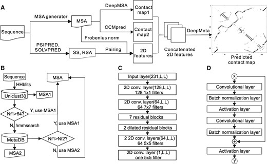
The architecture of the proposed methods. (A) is the flowchart of MapPred for contact map prediction. (B) is the MSA generator for constructing an MSA for a protein sequence. (C) is structure for the network used in the method DeepMSA. (D) is the structure for each residual block
Training and prediction are based on the dilated residual neural networks (ResNet) (Yu et al., 2017). We also tried other two variants of neural networks: convolutional neural networks (CNN) and common ResNet (He et al., 2016). Tests on the validation set (Supplementary Table S1) show that the common ResNet and the dilated ResNet consistently outperform the CNN. The dilated ResNet leads to slightly higher precision than the common ResNet. Thus the dilated ResNet is used here.
2.3 MSA generator
In this work, two databases are used for MSA generation. The first one is Uniclust30 (version 2017_10) with ∼13.6 million precompiled HMM profiles (Mirdita et al., 2017). The second one is an updated database from the work of (Ovchinnikov et al., 2017) (denoted by MetaDB). It currently includes about 7 billion unique sequences from the following resources: (i) JGI Metagenomes (7835 sets), Metatranscriptomes (2623 sets) and Eukaryotes (891 genomes); (ii) UniRef100; (iii) NCBI TSA (2616 sets); (iv) genomes collected from various genomic centers and online depositories (2815 genomes). Note that metagenomes and metatranscriptomes may contain noisy and fragmented sequences due to large-scale and high-throughput nature of the experimental setup. This may affect the quality of MSA and the final prediction results, which will be discussed experimentally later.
The search strategy works as follows (Fig. 1B). The HMM-HMM alignment program HHblits (Remmert et al., 2012) is first used to search against the Uniclust30 database, with at least 50% coverage and less than 0.001 e-value. The homologous sequences returned are used to construct the first MSA (denoted by MSA1). As in (Ovchinnikov et al., 2017), Nf is used to measure the depth of an MSA, which is defined as the number of non-redundant sequences at 80% sequence identity divided by the square root of the sequence length. When the Nf value of MSA1 is greater than 64 [this value was shown to be sufficient for accurate contact map prediction and subsequent structure prediction in Ovchinnikov et al. (2017)], the search is finalized and MSA1 is taken as the final MSA. Otherwise, the HMM-sequence alignment program hmmsearch (with default parameters) (Johnson et al., 2010) is used to detect homologous sequences in the MetaDB database. The returned sequences are used to construct the second MSA (denoted by MSA2), which is the final MSA if its Nf value is greater than 64. If Nf < 64 for both alignments, the one with the greater Nf is used.
2.4 Feature design
In the first stage of MapPred, the query sequence is submitted to the MSA generator to construct an MSA. Two contact maps are predicted from the MSA using DeepMSA and CCMpred. DeepMSA is a deep learning-based method developed in this work. It is an improved version of the DeepCov method, which uses only about half of the covariance features compared to the later and, as a result, enables large-scale training with a significantly reduced amount of computer memory and GPU time. CCMpred is a coevolution-based method, which is based on a pseudo-likelihood maximization approach, similar to GREMLIN but optimized for speed.
In the second stage, the final contact map is predicted with 11 2D channels, which are introduced below. The methods PSIPRED (version 4.01) and SOLVPRED (version 2.0.3) (Jones, 1999) are used to predict the secondary structure (SS) and the relative solvent accessibility (RSA), respectively. Each residue is encoded by four features, i.e. three probability values for secondary structure (α-helix, β-strand and random coil) and one for the solvent accessibility. These four 1D features (i.e. per residue) are converted into eight 2D channels (i.e. per residue pair) by concatenating the 1D features of the two paired residues. Another channel is the Frobenius norm matrix computed from the covariance matrices of the MSA. Together with the two 2D channels of the predicted contact maps in the first stage, 11 2D channels are obtained in total. These channels are fed into DeepMeta to predict the final contact map.
2.5 The DeepMSA method
We found two issues in this presentation of covariance. The first is about symmetry of matrix and the second is about the high number of matrices. Note that the protein contact map is symmetric as there is no order information for the residues at the positions i and j. However, the matrices derived from Eq. (1) are not symmetric. In addition, we observed that these matrices are often sparse and thus reduced the number by compressing those matrices based on the properties of amino acid groups (e.g. hydropathy index and side chain polarity). However, it did not achieve comparable performance to DeepCov, probably due to the loss of information.
In DeepMSA, the network (Fig. 1C) consists of the input layer, which contains 231 2D channels derived from the MSA, one 2D convolutional layer with 128 1 × 1 filters, one 2D convolutional layer with 64 7 × 7 filters, 7 residual blocks (Fig. 1D), two dilated residual blocks with a dilation ratio of 2, two 2D convolutional layers with 64 5 × 5 filters and one 2D convolutional layer with one 1 × 1 filter as the output layer. To reduce the training time and the computer memory, the batch size in each round is set to one, which enables training with proteins of varied lengths.
Note that there may be information loss by using Eq. (2). Thus, we also tried several other ways to reduce the number of channels and/or symmetrize the channel matrix. Tests on the validation set show that using Eq. (2) leads to very similar results as using all the 441 channels, but at significantly reduced computational cost (Supplementary Table S2).
2.6 The DeepMeta method
The network for DeepMeta is similar to the one used by DeepMSA. It consists of an input layer of 11 2D channels, one 2D convolutional layer with 32 7 × 7 filters, three residual blocks, two dilated residual blocks with a dilation ratio of 2, two 2D convolutional layers with 32 5 × 5 filters and one 2D convolutional layer with one 5 × 5 filter as the output layer. Because the number of channels is much smaller than that in DeepMSA, it is possible to train the network with a mini-batch weight updating mode, which is routinely used in the deep learning community.
However, the proteins have varied lengths and cannot be fed into the network directly. In our training dataset, the lengths are between 50 and 1000. We cut each input matrix into submatrices of fixed size, so that they could be simultaneously fitted into the network for contact map prediction; and then recover the full-size contact map by summing and averaging over the outputs from these submatrices.
The idea was illustrated in Supplementary Figure S1. A feature matrix F of size 5 × 5, is cut it into four 3 × 3 submatrices. A 3 × 3 window is moved on the matrix F with a step size of 3 by following a left-to-right and top-to-bottom order. When the window goes outside the boundary of F, it is returned back step by step until it fully fits into the matrix. The contact map for each submatrix is predicted independently, which is then merged together to generate the contact map for the original matrix. The appearing frequency for each element in the submatrices is counted, which forms a count matrix. The summations from the outputs of the submatrices are divided by the corresponding values in the count matrix to generate the final contact map. In this work, the size of the submatrix is 224, which equals to the medium value of the protein lengths in the training set. For small proteins with less than 224 residues, zeros were padded to the right-and-bottom edges to extend the matrix size to 224.
2.7 Performance evaluation
First, we define the gold standard for a residue-residue contact. Two residues are considered to be in contact if the Euclidean distance between their Cβ atoms (Cα atoms for glycine) is less than a specified threshold (8.0 Å). Depending on the separation (denoted by s) of two residues along the sequence, the contacts can be classified into three classes: short range (6 ≤ s < 12), medium range (12 ≤ s < 24) and long range (s ≥ 24). Short-range contacts are usually skipped as they are less useful for protein structure modeling.
The precision, i.e. the number of true positives divided by the number of predicted contacts, is used to measure the performance of a method. A predicted contacting pair is regarded as a true positive (TP) if the two residues are in contact in the native 3D structure. The top L/n ranked predictions are usually assessed, where the value of n can be 1, 2, 5 and 10. For the sake of simplicity, we mainly focus on the assessment for the top L/5 long-range predicted contacts. Switching to other L/n top-ranked predictions and/or the medium-range contacts does not change the major conclusions of this work. In the remaining of this paper, the precision is given for the top L/5 long-range predicted contacts by default, unless otherwise noted.
3 Results and discussion
3.1 Parameter optimization
The Keras (http://keras.io) and the Tensorflow libraries were used to implement our models. We initialized the weights as in He et al. (2015) and trained the networks from scratch. To train both DeepMSA and DeepMeta, the ReLU function (Nair and Hinton, 2010) is used for the intermediate layers and a sigmoid activation function is used at the very end to convert the predictions into probability values. The binary cross-entropy is used as the loss function. Because the contact map is usually sparse, we added the l1/l2 sparse function (Obozinski et al., 2008) to the loss function with a penalty coefficient of 2E-05. Test shows this sparse function improves the precision by about 2%.
DeepMSA was trained on a subset of the training set, consisting of 6289 sequences with length at most 500. After optimization, the hyper-parameters are as follows. Mini-batch size: 1; optimizer: SGD; learning rate: 0.1; weight decay: 1.5E-4; momentum: 0.95; and L2-norm regularization coefficient: 8E-5. Training of one model takes 15–20 epochs (around 12 h) to converge to a stable solution.
DeepMeta was trained on the entire training set of 6688 sequences. The hyper-parameters for DeepMeta are as follows. Mini-batch size: 8; Optimizer: SGD; learning rate: 0.02; weight decay: 1E-4; momentum: 0.95; and L2-norm regularization coefficient: 0.0004. Training of one model takes 25–35 epochs (around 5 h) to converge to a stable solution.
Due to the random effects in training, multiple models were trained for both DeepMSA and DeepMeta. The average of the predictions by the models is used as the final result. In our test, the usage of multiple models improves the precision by 3–5%. By default, multiple models were used unless noted.
To estimate the running time of the contact predictions, we randomly selected proteins with lengths between 50 and 1400. The MSAs of these sequences were submitted to MapPred. This was repeated by 20 times to collect the average running time. Here the I/O running time is not counted. Supplementary Figure S2 shows that running time on both GPU and CPU is quadratic to the sequence length.
3.2 Importance of the component features
There are three groups of features in MapPred: (1) CCMpred-based feature; (2) Sequence profile features, including SS, RSA and the Frobenius norm; and (3) DeepMSA-based feature. We use the validation set to analyze the importance of these feature groups. Supplementary Figure S3 summarizes the precisions for the models built with each feature group and their combinations. We can see that the precision for CCMpred is 54.83%, which is much lower than the precision (81.05%) for the deep learning model built with the feature group (3), and is higher than the precision (50.03%) for the deep learning model built with the feature group (2). Improvements were consistently observed when combining these features together. The most significant improvement was from the combination of the CCMpred and the second group of sequence profile features, with the respective precisions increased from 54.83% and 50.03% to 81.28%. This suggests that these two feature groups are largely complementary to each other. The best-performing method DeepMSA was also improved by 5% after combining with other features. The highest precision was observed when all three feature groups were combined together, which motivates us to use these combined features for building the MapPred model.
3.3 Comparison between DeepMSA and DeepCov
DeepMSA uses only about half number of the features from the method DeepCov, making it possible to train the models more efficiently. The performance of both methods on the benchmark datasets are summarized in Figure 2. DeepMSA consistently outperforms DeepCov by 10–13% for the three benchmark datasets. Head-to-head comparisons were presented in Figure 3, which indicates that DeepMSA outperforms DeepCov for most targets in each dataset.
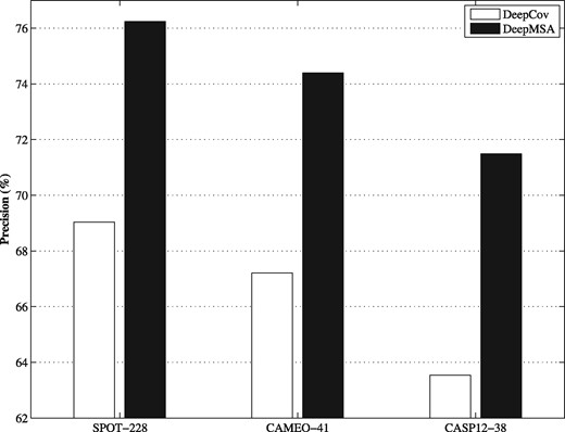
The comparison of DeepMSA with DeepCov on the three benchmark datasets
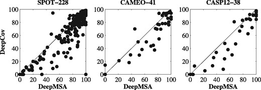
Head-to-head comparisons between the precisions (%) of DeepMSA and DeepCov on three benchmark datasets
Statistical tests were performed to estimate the significance level of the improvements as follows. For each benchmark dataset, we randomly split the set into two halves and then computed the average precision for each method. This experiment was repeated 100 times to generate 100 paired results. The Anderson-Darling test was first used to test whether the data follow a normal distribution at 0.05 significance level. The paired t-test was applied for a normal distribution. Otherwise, the nonparametric Wilcoxon signed-rank test was utilized. The P-value returned from the test indicates the significance level of the difference between two compared methods. In our experiments, the P-values are 7.24E-60, 1.07E-22 and 1.56E-20, for the SPOT-228, CAMEO-41 and CASP-38, respectively. Because the inputs are identical for both methods, the enhanced performance can be attributed to the improved feature design and the efficient training in DeepMSA.
3.4 Quality analysis of the metagenome sequence data
To investigate how the potential noise in metagenomic sequences could affect the performance of contact predictions, we enriched the HHblits alignments obtained on Uniclust30 with metagenomic sequences using varying bit score thresholds (from 0.2 to 1.2 times the length of the query protein). The lower the bit score is, the more metagenomic sequences are included in the alignment, on top of the Uniclust30 hits, gradually increasing the fraction of potentially noisy sequences in the resulting MSA. For the MSAs at each bit score threshold, we ran DeepMSA and assessed the precision of the predicted contacts on the three benchmark datasets. The results summarized in Figure 4 show that greater precision is achieved at smaller bit score thresholds. This suggests that it is valuable to uses metagenome sequences to generate MSAs, despite the potential noise in the dataset.
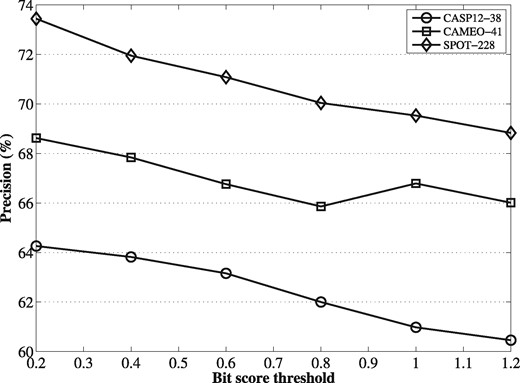
The precisions of DeepMSA on the benchmark datasets with MSAs enriched with metagenomic sequences at varying bit score thresholds
3.5 Contribution of the metagenome sequence data
In this study, the metagenome sequence database (MetaDB) was used together with Uniclust30 to improve the MSA generation. In this section, we investigate the contribution of the MetaDB to the contact map prediction as follows. For each target, we generated two sets of alignments to compare the contribution from the metagenome sequence data: one is purely from the Uniclust30 and the other is from MetaDB. To reduce the influence from other factors (e.g. accuracy in secondary structure prediction), two representative and clean methods are selected for this discussion: CCMpred and DeepMSA. The input to both methods is the MSA only, making them idea candidates for these experiments.
The results are summarized in Figure 5, which shows that on each benchmark dataset, greater precisions were achieved for both methods by using the MSAs from MetaDB. For CCMpred and DeepMSA, the respective improvements are in the 16–57% and 11–27% ranges. These data suggest that direct coupling-based methods depends more on the MSA quality than deep learning-based methods, consistent with the observation in the work on DeepCov. The P-values from statistical tests are listed in Supplementary Table S3 showing that the improvements by using the metagenome sequence data are significant (P-value < 1E-16).
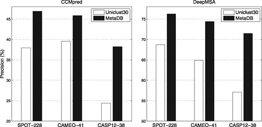
The precisions of CCMpred and DeepMSA on the benchmark datasets with MSAs generated from the Uniclust30 and the MetaDB databases
3.6 Comparison between MapPred and other methods
We compared MapPred with other methods on the benchmark datasets. The results are summarized in Table 1. The results for other methods on the SPOT-228 are cited from the work of SPOT-Contact. To compare with the latest versions of the two top-performing methods, SPOT-Contact and RaptoxX-Contact, we submitted the sequences of the CAMEO-41 and CASP12-38 datasets to the respective servers and assessed the precisions.
The comparison between the precisions (%) of MapPred and other methods
| Method | SPOT-228 | CAMEO-41 | CASP12-38 |
|---|---|---|---|
| R2C | 37.66 | NA | NA |
| DeepConPreda | 38.9 | NA | NA |
| CCMpred | 46.9 | 45.85 | 38.22 |
| NeBcon | 48.88 | NA | NA |
| MetaPSICOV | 50.07 | NA | NA |
| DNCON2 | 61.26 | NA | NA |
| DeepCov | 69.04 | 67.21 | 63.54 |
| MapPred | 78.94 | 77.06 | 77.05 |
| RaptorX-Contact | 78.3 | 81.57 | 75.8 |
| SPOT-Contact | 81.66 | 79.65 | 68.55 |
Note: The highest values are highlighted in bold.
On the SPOT-228 dataset, MapPred achieves 78.94% precision, comparable to those of SPOT-Contact and RaptorX-Contact (i.e. 81.66 and 78.3%, respectively). Except these two methods, MapPred outperforms other methods by a large margin. For example, MapPred’s precision is 14.3, 28.9 and 57.7% higher than DeepCov, DNCON2 and MetaPSICOV, respectively. On the CAMEO-41 dataset, MapPred’s precision (77.06%) is lower than those of RaptorX-Contact (81.57%) and SPOT-Contact (79.65%). On the CASP12-38 dataset, MapPred achieves the precision of 77.05%, which is slightly higher than RaptorX-Contact’s precision (75.8%) and significantly higher than SPOT-Contact’s precision (68.55%).
The lower precisions of MapPred compared with RaptorX-Contact and SPOT-Contact on the CAMEO-41 and the SPOT-228 datasets may be partly explained by the more stringent criteria used in the construction of our training set. In these two methods, the sequence identity cutoff between the training and test proteins was 25% and the profile-sequence alignment tool PSI-BLAST was used to exclude similar proteins in the training set. In comparison, the sequence identity cutoff here is 20% and the more sensitive profile-profile alignment algorithm HHsearch was used to filter out proteins from the training set. When the same standards were used, we observed an increased size of the training set. The precision gap between our method and these two methods becomes smaller after re-trained on the new training set.
Supplementary Figure S4 shows head-to-head comparisons between MapPred and RaptorX-Contact on the CAMEO-41 and CASP12-38 datasets. On these two datasets, there are about 1/3 targets that MapPred outperforms RaptorX-Contact and 1/3 targets that both methods have similar precisions. This suggests that MapPred is complementary to RaptorX-Contact and a combination of them should be able to improve the predictions further.
To demonstrate that the improvement of MapPred over other methods is not completely due to the usage of the metagenomic sequences, we did the following experiment on the CASP12-38 dataset. The MSA for each target in this dataset was generated by searching against the sequence database uniprot20_2016_02 (before the date of CASP12) using HHblits at 50% coverage and 0.001 e-value. With this new alignment, the precision of MapPred drops to 60.31%; but is significantly higher than the top value (47.09% by RaptorX-Contact) listed on the CASP12 website. This suggests that besides the metagenomic sequences, other factors such as the improved feature design and the training by ResNet also contribute to the success of MapPred.
3.7 Performance of MapPred in the blind tests of CASP13
With MapPred, we participated in the contact prediction category of the CASP13 experiment with the group name Yang-Server (group code RR164). The Z-scores over 31 free-modeling domains shows that our method is ranked at the 9th out of 46 participating groups. When ranking by the average precision of the top L/5 long-range predictions, our method is at the 7th. When more predictions are assessed, the ranking of our method is improved and the gap with the top-ranked method becomes smaller. For example, when the top L long+medium-range predictions are assessed, our method is ranked at the 5th (Supplementary Fig. S5). After CASP13, a few critical bugs were found in the version used during the CASP13 experiments. We re-trained MapPred after fixing these bugs. Test on these 31 targets (with the same MSAs used by Yang-Server) suggests that the top L/5 long-range precision was improved from 60.156% (for Yang-Server) to 69.79%, very close to that of RaptorX-Contact (70.054%). Supplementary Figure S6 shows that the improved MapPred is complementary to RaptorX-Contact. In comparison, the precision for the method SPOT-Contact (the top method on the dataset SPOT-228) is 58.09% (collected from the CASP13 website), which is lower than both the old and the new versions of MapPred.
4 Conclusions
The precision of protein contact map prediction is constantly improving in recent years, due to the continuous accumulation of sequence data and the development of deep learning algorithms. In this work, we presented MapPred, a new method for protein contact map prediction that consists of two component methods, i.e. DeepMSA and DeepMeta. Using the improved metagenome data-derived MSAs, we first developed a deep learning-based method DeepMSA, which only relies on the MSA as the input. Then a deep-learning based meta predictor DeepMeta was developed by combing DeepMSA with a direct-coupling method CCMpred. We demonstrated that the vast sequence data from the metagenome sequencing projects result in improved protein contact map predictions with the residual neural networks. Experiments on three benchmark datasets show that our method is complementary and comparable to the state-of-the-art methods. We attribute the success of MapPred to the usage of the metagenome sequence data, the improved feature design in DeepMSA and the optimized training with the residual neural networks. In the near future, the predicted contacts will be used to guide the Rosetta de novo structure modeling, to investigate how much deep learning-based predictions could add on top of the coevolution-based predictions.
Funding
The work was supported in part by National Natural Science Foundation of China (NSFC 11871290 and 61873185), the Fundamental Research Funds for the Central Universities, Fok Ying-Tong Education Foundation (161003), China Scholarship Council, KLMDASR and the Thousand Youth Talents Plan of China.
Conflict of Interest: none declared.
References

