MetaBMF: a scalable binning algorithm for large-scale reference-free metagenomic studies

Abstract

Motivation

Metagenomics studies microbial genomes in an ecosystem such as the gastrointestinal tract of a human. Identification of novel microbial species and quantification of their distributional variations among different samples that are sequenced using next-generation-sequencing technology hold the key to the success of most metagenomic studies. To achieve these goals, we propose a simple yet powerful metagenomic binning method, MetaBMF. The method does not require prior knowledge of reference genomes and produces highly accurate results, even at a strain level. Thus, it can be broadly used to identify disease-related microbial organisms that are not well-studied.

Results

Mathematically, we count the number of mapped reads on each assembled genomic fragment cross different samples as our input matrix and propose a scalable stratified angle regression algorithm to factorize this count matrix into a product of a binary matrix and a nonnegative matrix. The binary matrix can be used to separate microbial species and the nonnegative matrix quantifies the species distributions in different samples. In simulation and empirical studies, we demonstrate that MetaBMF has a high binning accuracy. It can not only bin DNA fragments accurately at a species level but also at a strain level. As shown in our example, we can accurately identify the Shiga-toxigenic Escherichia coli O104: H4 strain which led to the 2011 German E.coli outbreak. Our efforts in these areas should lead to (i) fundamental advances in metagenomic binning, (ii) development and refinement of technology for the rapid identification and quantification of microbial distributions and (iii) finding of potential probiotics or reliable pathogenic bacterial strains.

Availability and implementation

The software is available at https://github.com/didi10384/MetaBMF.

1 Introduction

Accumulating evidence suggests that inhabiting microbial communities in human intestine, skin, oral cavity and genitourinary tract play a crucial role in human health (Gerritsen et al., 2011). Disruption of these delicate ecosystems can cause some perplexing diseases including asthma (Huang and Boushey, 2015), allergies (Huang et al., 2017), obesity (Turnbaugh et al., 2006), diabetes (Brown et al., 2011), autoimmune diseases (Severance et al., 2016) and perhaps even autism (Clemente et al., 2012). Thus, understanding the microbial community is very important for identifying disease-related pathogens and finding their potential treatment strategies.

Moreover, an understanding of the microbial ecosystem is not only important in medical research but is also important in marine research (Hentschel et al., 2012), biothreat detection (Gardner et al., 2015), biofuel study (Xing et al., 2012) and global warming (Zhou et al., 2012). Besides the scientific study, a clear understanding of the microbial system has also been shown to be useful in an industry setting as described in the following two examples. (i) It can be used as a simple research tool for the study of bacterial metabolism and as an easy method for the optimization of bacterial production of fine chemicals or other fermentation processes. (ii) It can be used by manufacturers to control the bacterial contamination in food products in order to meet stringent regulations of the food industry.

Despite its importance, our understanding of the microbial ecosystem is severely limited by the difficulty in cell culturing and separation, the need for highly trained laboratory personnel and the requirement of expensive and high-maintenance equipment. The biodiversity of the microbial ecosystem has been barely studied, not to mention interactions between microbial species. However, this dilemma can be overcome by recently developed DNA sequencing technology. By sequencing bulk DNA that is directly extracted from environmental samples, one can bypass all the aforementioned difficulties and easily obtain the DNA fragments or short reads of every genome in the microbial system. This type of research is referred to as a metagenomic study. The segmentation of DNA fragments or short reads either according to their similarities to some known reference genomes or according to their composition similarities [e.g. similarities k-mer distributions (Teeling et al., 2004)] is referred to as metagenomic binning. In general, metagenomic binning is similar to sorting puzzle pieces and assembling multiple puzzles simultaneously.

Although this line of research holds tremendous scientific promise, the delivery of this promise, however, has not yet been fully materialized, mainly because of the lack of effective and efficient bioinformatics tools for binning billions of mixed short reads into multiple genomes. One major challenge arises from the incredible complexity and heterogeneity of genomes in the samples. Reference-based binning methods such as MAGEN (Huson et al., 2007), MetaPhyler (Liu et al., 2010), Kraken (Wood and Salzberg, 2014) and CLARK (Ounit et al., 2015) require us to know the reference genomes (‘template of puzzles’) of the interested microbial species, which are not available most of the times. The composition similarity based methods are reference-free. However, the composition similarity based methods cannot separate genetically similar genomes and thus can only obtain a separation at a high taxonomy rank such as the genus level. In order to improve k-mer-based approaches, coverage-based methods such as CONCOCT (Alneberg et al., 2014), MaxBin (Wu et al., 2016), MetaBAT (Kang et al., 2015), Groopm (Imelfort et al., 2014) and VizBin (Laczny et al., 2015) are developed to integrate the coverage information (i.e. the average number of short reads covering each base pair of a contig after alignment) with sequence composition information such as k-mer distribution. However, they are usually very slow and a large-scale study of these methods are infeasible. To overcome the aforementioned challenges, an innovative approach MetaGen is proposed in Xing et al. (2017), which models the relative abundance from multiple samples as a mixture of multinomial distribution and cluster DNA fragments using EM algorithm. Although MetaGen achieves high binning accuracy, even for genetically similar microbial strains, the EM algorithm used in Xing et al. (2017) suffers from high computational and memory costs. It can fail from a memory overflow with thousands of samples. To adapt MetaGen for massive metagenomic applications, we developed a powerful and fast reference-free binning tool MetaBMF. The proposed method enjoys both high binning accuracy and fast computation, which are essential for large-scale metagenomic applications. It is especially important for rapid and reliable detection and characterization of microbial pathogens, particularly previously unknown ones, to human or animals. Our efforts on metagenomic binning will lead to (i) fundamental advances in metagenomic studies and (ii) a novel method for timely detection of pathogenic bacteria.

In addition to biological achievement, the estimation method that we developed is a major technological breakthrough. We can reduce the current computational speed from a polynomial order to a linear order, which is almost the fastest speed that one can achieve. The software is available at https://github.com/didi10384/MetaBMF.

2 Materials and Methods

MetaBMF targets on large-scale biomedical studies where species in each sample have different distributions. This assumption can be satisfied in most scientific studies. For example, we can safely assume that the microbial distributions in the human gut are different for different subjects. Under this assumption, we can safely assume that the cross-sample relative abundance of one species is different from that of another given species. Since the relative abundance of a contig equals the relative abundance of the species that contain it, we can make use of the relative abundance of each species across samples to sort contigs based on the fact that contigs from different species have different relative abundances across samples.

2.1 Model setup

Let us consider the metagenomic sequencing data consisting of short reads from the genomes of the organisms collected from each sample. To control the binning error caused by the sequencing bias and error and to improve the binning accuracy for species that are rare in some samples, we first conduct a pooled assembly by connecting overlapped short reads from all samples into longer contigs. Assume that n contigs were obtained from p metagenomic samples, with a total of K species involved, we can generate a n by p read counts mapping matrix X, with its (i, j)th entry recording the number of short reads from the jth sample mapped onto the ith contig.

Let B_ik be the binary membership labeling variable such that B_ik = 1 if contig $i\in$ species k, and P_kj is the abundance of species k in sample j. Then, the sequencing depth of the ith contig in sample j is ${\sum }_{k=1}^K{B}_{\mathit{ik}}{P}_{\mathit{kj}}$⁠, and the relative abundance of mapped reads counts $\mathrm{ }{x}_i=(X_{i1},\dots ,X_{\mathit{ip}})$ is proportional to $p_k=(P_{k1},\dots ,P_{\mathit{kp}})$ if contig $i\in$ species k. The proportion is the average number of short reads that contig i can generate and is related to contig length. Consequently, as shown in Fig. 1, if we ignore any measurement errors, the read count mapping matrix X can be decomposed into three factors: a normalization matrix Λ, a signature matrix B and a relative abundance matrix P. That is

$$X=\Lambda \mathit{BP},$$

(1)

where Λ is a n × n nonnegative diagonal matrix with the ith diagonal entry being proportional to the length of the ith contig, B is a n × K binary matrix with the ikth entry indicating whether the ith contig comes from the kth species and P is a K × p nonnegative matrix with the kjth entry being the cross-sample relative abundance of species k in sample j. In real practice where sequencing error, sequencing bias a and assembly error exist, we will estimate Λ, B and P by minimizing

$$L(\Lambda ,B,P)=\left|\right|X-\Lambda \mathit{BP}|{|}_F,$$

(2)

where $\left|\right|·|{|}_F$ represents the Frobenius norm.

Fig. 1.

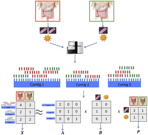
MetaBMF pipeline: first, DNA from two pseudo-metagenomic samples, of which the relative abundance is 2:1 for species one and 1:1 for species two are sequenced by the sequencing machine. Second, short reads are assembled into contigs by pooling all reads from the two samples and generating the read count mapping matrix X. Third, obtain the normalization matrix Λ, the signature matrix B and abundance matrix P using our novel binary matrix factorization algorithm

2.2 Stratified angle regression algorithm for binary matrix factorization

Unlike all existing binning methods, which aim to find the optimal partition of contigs among all $\left(\begin{array}{c}{2}^n\\ K\end{array}\right)$ candidate partitions, we aim to find K seed contigs that belong to K different species and then assign the rest of the contigs according to their cross-sample distributional similarities with the K seed contigs.

We first found K contigs which distributed very differently in samples and define a set $\mathcal{S}$ which include all their indices. As the relative abundance of a contig equals the relative abundance of its corresponding species, we can use the cross-sample relative abundance of the K seed contigs as an estimate of the species’ cross-sample relative abundance P. When the relative abundance P is known, the rest of the n − K rows of B can be obtained by conducting a linear regression

$$\frac{x_{\ell }^{\prime }}{\left|\right|x_{\ell }^{\prime }|{|}_1}=P\prime B_{\ell }^{\prime }+{ϵ}_{\ell },$$

(3)

where $\left|\right|·|{|}_1$ denotes the L₁ norm of a vector, $x_{\ell }$ is the $\ell$th row of the read count mapping matrix X, $B_{\ell }$ is the $\ell$th row of the signature matrix B and ${ϵ}_{\ell }$ is the stochastic error. Without any constraint on B, an optimal estimate of $B_{\ell }$ can be achieved by minimizing the least square functional $L(B_{\ell }^{\prime })=\left|\right|\frac{x_{\ell }^{\prime }}{\left|\right|x_{\ell }^{\prime }|{|}_1}-P\prime B_{\ell }^{\prime }|{|}_2$⁠. However, this approach does not work for our model because $B_{\ell }^{\prime }$ is a binary vector. Moreover, contig $\ell$ can only belong to one species. Thus, only one column of $P\prime$ has a nonzero coefficient. This is the column that is most correlated with the response variable $x_{\ell }^{\prime }$⁠. Let k denote the index of this column or the corresponding row of P. Then, the kth element of $B_{\ell }$ equals to one and the rest of K−1 elements equal to zero. Because the algorithm estimate the $\ell$th row of B by calculating the angle between $x_{\ell }$ and rows of P, we refer to the proposed algorithm as the stratified angle regression (SAR) algorithm.

The strategy for MetaBMF, an algorithm based on the SAR algorithm, can be sketched in three steps. First, we find K seed contigs for K species. Second, we estimate the cross-sample relative abundance of each species by its corresponding seed contigs. This can be easily achieved as the relative abundance of contigs and species are the same. Third and the most important step is to assign each of the rest of the n − K contigs to their associated bins using the SAR algorithm. Compared with existing matrix factorization methods, MetaBMF can greatly reduce the computational complexity and is more applicable in a big data setup. It can easily bin more than 500 000 contigs in a few seconds.

2.3 Implementation

This section consists of two subsections. In the first section, we proposed a strategy to select the K seed contigs and in the second section, we proposed an estimation method for the number of species K.

2.3.1 Selecting the set of seed contigs

To select the seed contigs, we start with the contig with the largest $\left|\right|x_i|{|}_2$ and sequentially add an additional contig to the collection. The procedure terminates when K seed contigs are obtained.

Let $\mathcal{A}$ denote the collection of row indexes of X and ${\mathcal{A}}_k$ the collection of row indexes that corresponding to the current selected k seed contigs. To add additional seed contigs to ${\mathcal{A}}_k$⁠, we need to define the following distance function:

$$d_{\mathit{ii}\prime }=1-\frac{<x_i,x_{i\prime }>}{\left|\right|x_i\left|{|}_2\right|\left|x_{i\prime }\right|{|}_2}$$

(4)

to quantify the distributional difference of two contigs where $<·,·>$ is the inner product of two vectors and $\left|\right|·|{|}_2$ is the Euclidean norm. Recall that we assume the cross-sample distribution for a given species is unique. It is easy to see that $d_{\mathit{ii}\prime }$ is near 0 if contig i and $i\prime$ belong to the same species, and $d_{\mathit{ii}\prime }$ is away from 0 if contig i and $i\prime$ are from different species. The larger the $d_{\mathit{ii}\prime }$ is, the more unlikely contigs i and $i\prime$ are in the same species.

Then, we come up with the following criteria. For any $i\prime \in \mathcal{A}/{\mathcal{A}}_k$⁠, we define the smallest distance function

$$\text{SD}\left(i\text{'}\right)=\underset{i\in {\mathcal{A}}_k}{\min }{d}_{\mathit{ii}\text{'}}$$

(5)

and the new seed contig i₀ should be the maximizer of $\text{SD}(i\prime )$⁠, i.e. $i_0=\text{arg}\hspace{0.17em}\hspace{0.17em}{\text{max}}_{i\prime \in \mathcal{A}/{\mathcal{A}}_k}\text{SD}(i\prime )$⁠. We add new seeds sequentially until $\left|{\mathcal{A}}_k\right|=K$⁠, i.e. the total number of seeds approaches K.

2.3.2 Estimate the number of species K

To determine K, we adopt the silhouette statistic that is proposed by Rousseeuw (1987). For any given K between 1 and D, where D is a crude upper bound of K chosen by users, we estimate P, B and Λ using SAR with K number of species. Suppose that ${\mathcal{S}}_k$ is the collection of contigs for species k that is obtained by SAR and the cardinality of ${\mathcal{S}}_k$ is n_k. Based on the current partition$({\mathcal{S}}_1,\dots ,{\mathcal{S}}_K)$⁠, we can evaluate the within-group divergence for contig i by

$$a_i(K)=\frac{1}{n_k}\sum _{i\prime \in {\mathcal{S}}_k}{d}_{\mathit{ii}\prime },$$

(6)

and the between-group divergence by

$$b_i(K)=\underset{k\prime \ne k}{\min }\frac{1}{n_{k\prime }}\sum _{i\prime \in {\mathcal{S}}_{k\prime }}{d}_{\mathit{ii}\prime },$$

(7)

if contig i is in group k. It was shown in Rousseeuw (1987) that the silhouette statistics based on $b_i(K)$ and $a_i(K)$ can be used as an consistent estimate of K. Define

$$C(K)=\frac{1}{n}\sum _{i=1}^n\frac{b_i(K)-a_i(K)}{\max (a_i(K),b_i(K))}.$$

(8)

We choose $K_{\mathit{opt}}=\arg {\max }_{1\le K\le D}C(K)$⁠. Heuristically, when between-group divergence is bigger than the within-group divergence, the addend in Eq. (8) is increasing as $a_i(K)/b_i(K)$ is decreasing for better classification. Consequently, C(K) is increasing. However, if K is too big, we may mistakenly split one species into two species. The between-group divergence is more similar to the within-group divergence for the mistakenly split groups. Consequently, $b_i(K)-a_i(K)$ will be close to zero for many i and C(K) starts to decrease, which suggests that we need to reduce K. Our extensive simulation study shows that C(K) is a consistent estimator of K and can be generally used in practice. In Fig. 2, we plot the silhouette statistics for data with 50, 100 and 150 species. Clearly, C(K) is maximized at 50, 100 and 148, which provides a satisfactory estimate of the number of species in the study. In large-scale metagenomic studies, the number of species usually ranges from hundreds to thousands. We recommend setting a wide searching range of K and a large step size and then refine the search with a small step size. For example, we could search K in $(100,200,300,\dots ,3000)$⁠. Once we have a rough estimate of K_opt such as $K_{\mathrm{opt}}\in \left(\mathrm{1000,1200}\right)$⁠. Then we will refine the search in (1000, 1200) with a small step size. This searching strategy will significantly reduce the computation time (also see our software manual for details).

Fig. 2.

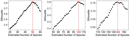
Silhouette statistic under different estimation of number of species. The selected number of species are 50, 100 and 148, respectively, when the true number of species are 50, 100 and 150

2.4 MetaBMF algorithm

MetaBMF is a complete computational pipeline for large-scale multi-sample metagenomic analysis. It integrates genome assembly methods, a two-step binary matrix factorization algorithm (SAR), and the number of species estimation method for simultaneous estimation of species compositions and distributions. Our procedure starts at a carefully selected K row of X, of which the normalization can be used as an estimate of the cross-sample relative abundance P. We then fill $B_{\ell k}$⁠, one of the rest n − K rows, by one if the maximum correlation is obtained between the kth row of P and the $\ell$th row of X or by zero otherwise. The norm of $x_{\ell }$ fills the $\ell \ell$th diagonal element of Λ. Finally, we calculate C(K) and update K by K + 1 until the maximum C(K) is obtained. Below we summarize the MetaBMF algorithm.

Algorithm 1.

MetaBMF

Step 1: Assemble short reads from pooled samples into contigs using genome assembly software such as Ray-assembler or MegaHIT.

Step 2: Construct the read count mapping matrix X, which is the input of the SAR algorithm.

while K < D do

 Step 3: Sequentially select the seed contigs one at a time by maximizing the smallest distance function $\text{SD}(·)$⁠.

 Step 4: Normalize the seeds by their L₁ norm and then fill into the row of P. Denote the estimated P by $P^{(K)}$⁠.

 Step 5: Apply SAR sequentially to $x_{\ell }$ for $\ell \in \mathcal{A}/{\mathcal{A}}_K$ and replace the $\ell$th row of B by $B_{\ell }$⁠. Denote the estimated B by $B^{(K)}$⁠.

 Step 6: Fill in the diagonal element of Λ by L₁ norm of the corresponding row of X. Denote the estimated Λ by ${\Lambda }^{(K)}$⁠.

 Step 7: Calculate C(K) and update K by K + 1 if $C(K)>C(K-1)$ otherwise output ${\Lambda }^{(K-1)},\hspace{0.17em}{B}^{(K-1)}$ and $P^{(K-1)}$⁠.

end while

2.5 Computational complexity

As with all binning methods, MetaBMF consists of two building blocks, assembling short reads into contigs and binning contigs, both of which have their own computational complexity. However, the major contribution of MetaBMF is in the contig binning step. Thus, we will focus our discussion on contig binning (Steps 3–7 of Algorithm 1) in this section. In fact, we can show that the computational complexity of Steps 3–7 is linear in n (number of contigs), which facilitate the application of MetaBMF in large-scale metagenomic studies that cannot be easily handled by other methods. As illustrated in Algorithm 1, maximizing the smallest distance function in Step 3 takes $O(\mathit{np}{K}^2)$ flops and to solve n linear programmings in Steps 4–7 requires $\max (O(n{p}^{2}K),O(\mathit{np}{K}^2))$ flops. Notice that step 5 is fully parallelizable. We can use distributed algorithms to further accelerate the computation. As the number of samples p and the number of species K are nearly negligible compared to the number of contigs n, the total computational cost of the binning step is linear in n.

3 Results

3.1 Simulation studies

To investigate how binning accuracy was affected by different parameters, such as the sequencing depth, the number of samples and the number of species, we conducted extensive simulations to compare MetaBMF with three state-of-the-art reference-free binning methods: CONCOCT, MaxBin and MetaBAT, and one reference-based method, CLARK. The candidate species (or strains) that we used in this simulation can be downloaded from Supplementary Tables S1–S3 in Xing et al. (2017). Because all the methods except MetaBMF can be significantly impaired for contigs shorter than 1000 bps, we used only the subset of contigs with a length longer than 1000 bps for CONCOCT, MetaBMF, MaxBin and CLARK to facilitate a fair comparison. For MetaBAT, we used contigs longer than 1500 bps, which is the default minimum length for contigs that can be used in MetaBAT.

3.1.1 Change of binning accuracy for varying number of species

Short reads from K species mixed in a randomly generated proportional distribution were independently simulated for each of the 80 samples at a pooled sequencing depth 120× (or 1.5× per sample), where K varies from 50 to 150 with each time increased by 50. The per-species coverage decreases when the number of species increases. As shown in Fig. 3, the binning accuracy for all the methods except MetaBMF and Clark decreases drastically. The performance of MetaBMF and Clark is robust when the number of species is large. Notice that all the genomes from which the simulated short reads are generated have reference genomes in the database, which give a significant advantage to the reference-based binning method CLARK. Thus, CLARK should provide almost the golden standard binning result. However, as one can see from Fig. 3, the binning accuracy for MetaBMF is comparable to CLARK for all simulated data and is better for 150 species, though MetaBMF is a reference-free binning method.

Fig. 3.

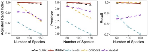
Adjusted Rand Index, Precision and Recall of CLARK, MetaBMF, MaxBin, CONCOCT and MetaBat evaluated under different number of species for 120× sequencing depth and 80 samples

3.1.2 Change of binning accuracy for varying number of samples

In this example, we simulated short reads using the same strategy as the previous example. However, we have changed the sample size from 20 to 80 while fixing the number of species to be 100. As shown in Fig. 4, the binning accuracy decreases for an increased sample size. This is well expected as the per-sample sequence depth decreases for an increased number of samples. Similar to the previous example, the performance of MetaBMF and Clark is all close to perfect, which ensures that one can safely use MetaBMF even when reference genomes are available.

Fig. 4.

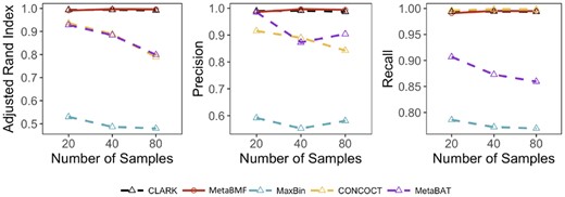
Adjusted Rand Index, Precision and Recall of CLARK, MetaBMF, MaxBin, CONCOCT and MetaBat evaluated under different number of samples for 120× sequencing depth and 100 species

3.1.3 Change of binning accuracy for varying sequencing depths

As in the previous two examples, we simulated short reads for $80\times ,\hspace{0.17em}120\times$ and $160\times$ pooled sequencing depths with 80 samples and 100 species. Unlike the previous two examples, the binning accuracy increases for all methods under this setup. As shown in Fig. 5, MetaBMF and Clark are almost perfect even when the average per-sample coverage is around $1\times$⁠. This ensures that MetaBMF has consistent performance even at a fairly low coverage level.

Fig. 5.

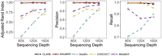
Adjusted Rand Index, Precision and Recall of CLARK, MetaBMF, MaxBin, CONCOCT and MetaBat evaluated under different sequencing depths for 100 species and 80 samples

In Fig. 6, we illustrate the binning results for a setup with 100 species, 80 sample and $120\times$ coverage levels. Different species are represented by different colors and each binned contig is represented by a bar in the graph. Bars with uniform color indicate no binning error. It is easy to see that MetaBMF has a pretty high binning accuracy. Clark, although having similar binning accuracy as MetaBMF for bins with a large number of contigs, tends to produce species with only one or two contigs due to the error generated by mapping contigs to their reference genomes. Compared to MetaBMF and Clark, other methods are more error-prone.

Fig. 6.

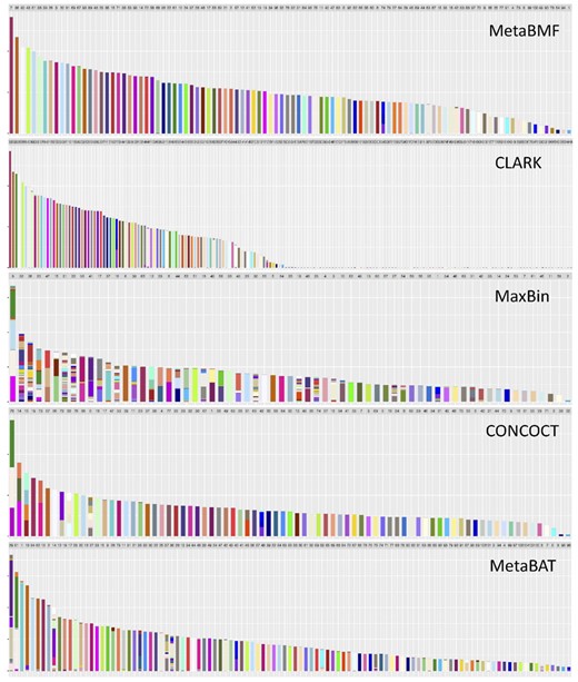
Binning results for MetaBMF, CLARK, MaxBin, CONCOCT and MetaBAT for data with 120× sequencing depth, 80 samples and 100 species. Each bar represents one bin obtained using the corresponding binning method. The color of a bin should be the same if there is no binning error. (Color version of this figure is available at Bioinformatics online.)

3.1.4 Computational time

In addition, we compare the computational time of MetaBMF with MaxBin, CONCOCT and MetaBAT. The computation has been done on a computer node with Intel(R) Xeon(R) CPU E5-2690 v3 @ 2.60 GHz and 256 Gb RAM. We set parameters to maximize the utilization of the computational resource for all the methods. As shown in Fig. 7, the computational time of MetaBMF is the lowest in all settings. In average, MetaBMF is $35\times$ faster than the second fast method, MetaBAT. Also there are less than $2\times$ increment of computational when the sequence depth, number of sample and number of species increase from low to high.

Fig. 7.

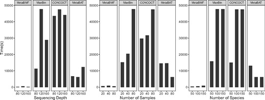
Computational time for MetaBMF, MaxBin, CONCOCT and MetaBAT for varying sequence depth (left panel), varying number of samples (middle panel) and varying number of species (right panel)

3.1.5 Assembly of metagenomic samples

The binning algorithm is based on the assembled genomic fragments. The question then arises: does the choice of assembler affect the binning accuracy? We then test the four reference-free binning methods using two different assemblers: Ray (Boisvert et al., 2012) and MegaHIT (Li et al., 2015) on the simulated dataset with 80 samples, 100 species and $120\times$ sequencing depth. As shown in Fig. 8, CLARK and MetaBAT perform better when using Ray-assembler; CONCOCT and MaxBin have better performance when using MegaHIT assembler; MetaBMF has the similar performance based on these two assemblers. The result shows that MetaBMF is least affected by the use of assembler. Also note that MetaBMF is also compatible with other assemblers, which is documented in our software manual.

Fig. 8.

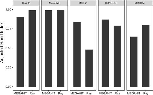
Adjusted Rand Index of CLARK, MetaBMF, MaxBin, CONCOCT and MetaBAT are evaluated using two different assemblers, MegaHIT and Ray on simulated dataset with 80 samples, 100 species and $120\times$ sequencing depth

3.2 Metagenomic analysis of 2011 German Escherichia coli outbreak

The outbreak of Shiga-toxigenic Escherichia coli (STEC) O104: H4 in Germany caused an economic loss of $\$200$ million per week for Spanish exporters and infection of 3950 people with 53 deaths. This devastating pandemics can be avoided with prompt and accurate microbial identification methods. In fact, the social and economic losses from the outbreak can be greatly reduced if the pathogenic bacteria, enteroaggregative E.coli (EAEC) strain that presented itself in organic fenugreek sprouts was not misdiagnosed as enterohemorrhagic E.coli strain originating from Spanish cucumbers. However, due to the experimental and technological difficulties, many existing metagenomic methods can only identify microbial organism at best at species level. The major challenges are that the two strains are highly genetically similar. In this example, we show that MetaBMF can promptly and accurately identify the pathogens at a strain level because we do not use the sequence similarity for pathogen identification.

In Loman et al. (2013), DNA samples were extracted from the feces of 43 STEC-positive and 10 STEC-negative patients who suffered from diarrhea during the STEC O104: H4 outbreak, and over 3 billion 150-bp reads were generated by Illumina high-seq 2500 sequencer. Using Ray-assembler, we obtained $\sim 75$K contigs that are longer than 1000 bps and shared by at least 15 patients. As shown in Fig. 9A, the 75 K contigs are binned to 450 candidate microbial units by MetaBMF. Figure 9B demonstrates that the number of significant microbial species of STEC-positive group is larger than that of STEC-negative group. Among the 450 candidate microbial units, only the unit (Fig. 10) corresponding to EAEC strain have significantly different abundance between STEC-positive patients and STEC-negative patients by Wilcoxon-rank sum test at a 5% false discovery rate, which confirms that MetaBMF can indeed find the pathogenic strain.

Fig. 9.

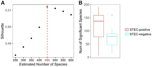
Plotted in (A) is the C(K) versus K. Because C(K) is maximized at 450, we let K = 450. In (B), we plot how the number of significant species distributed among 43 STEC-positive samples (left red boxplot) and 10 STEC-negative samples (right blue boxplot). (Color version of this figure is available at Bioinformatics online.)

Fig. 10.

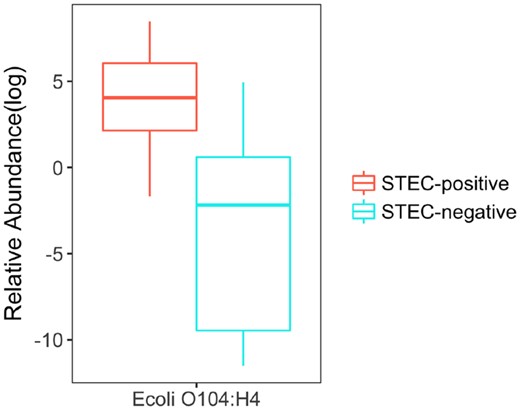
Relative abundance of E.coli O104: H4 which has significant differences between STEC-positive samples (left red box) and STEC-negative samples (right blue box). (Color version of this figure is available at Bioinformatics online.)

A predictive model with 450 microbial units was built by logistic regression with LASSO penalty (Tibshirani, 1996) to ease the diagnostic of STEC infection. The 5-fold cross-validation (CV) of the mis-diagnostic error is 0.094 with the area under receiver operating curve (AUC) being 0.901 for all the 53 patients.

3.3 Metagenomic analysis of coronary heart disease

Coronary heart disease (CHD) is the most common type of heart disease in the world that is caused by a buildup of plaque, which comes from cholesterol and other substances deposited in the artery. This deposit causes a narrowing of the artery, resulting in limited blood flow, which causes chest pains and shortness of breath, eventually leading to heart attack and death. Accumulating evidence has revealed that intestinal microbiota plays an important role in regulating metabolism-dependent pathways such as the trimethylamine N-oxide pathway, short-chain fatty acids pathway and primary and secondary bile acids pathways. Consequently, understanding the bacterial composition and distribution in CHD patients play a pivotal role in understanding CHD.

In this study, we conduct a thorough metagenomic analysis on CHD using MetaBMF and data collected by Feng et al. (2016). DNA samples were extracted from the feces of 59 CHD patients and 43 control patients, and sequenced using illumina high-seq 2000 which generated 2 G short reads. Using this data, we assembled the short reads by Ray-assembler which generated 5 M contigs. Deleting contigs with low sequence depth, contigs that are shorter than 1000 bps and contigs that are shared by <30% of individuals, we obtained 250 K contigs. For each contig, we searched the NCBI nucleotide database and used TAXAassign (https://github.com/umerijaz/TAXAassign) to assign it to a taxonomic group. Only 8.3% of the contigs could be assigned at the species level and 14.3% could be assigned at the phylum level. Roughly 85.7% of contigs could not be mapped to any reference genomes even at the phylum level. Thus, reference-free binning methods are highly desirable for this data.

We applied MetaBMF to bin the 250 K contigs and obtained 2200 species (see Fig. 11A), among which 170 are literally known species. Figure 11B demonstrate that the number of significant microbial species varies more in CHD group than in control group. A species was treated as a significant species if its scaled relative abundance is larger than 0.1%. Using a Wilcoxon-rank sum test (Haynes, 2013), we identified 21 species that distributed significantly in the CHD group and control group with a 5% false discovery rate. Among the 21 identified species, 10 of them are literally known.

Fig. 11.

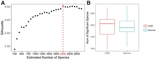
Plotted in (A) is the C(K) versus K. Because C(K) is maximized at 2200, we let K = 2200. In (B), we plot how the number of significant species distributed among 59 CHD patients (left red boxplot) and 43 control subjects (right blue boxplot). (Color version of this figure is available at Bioinformatics online.)

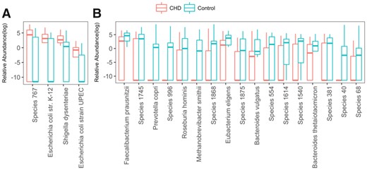
We listed species that are more likely to appear for CHD patients in Fig. 12A and for healthy subjects in Fig. 12B. The results that we obtained are consistent with the published works for known species. The significantly high abundance of E.coli strain K-12 and strain UPEC, as well as Shigella dysenteriae in CHD patients were also observed by Jie et al. (2017). Figure 12A suggests that the listed four microbial species are positively associated with CHD. Alternatively, we also found 17 species that might be used as probiotics for CHD, where four of them are well-known to be negatively correlated with CHD risk factor including Faecalibacterium prausnitzii, Roseburia hominis, Methanobrevibacter smithii and Bacteroides thetaiotaomicron. A decrease of F. prausnitzii can significantly increase serum TMAO, a pro-atherogenic compound, and a decrease of R. hominis can increase the risk of ulcerative colitis, a well-known risk factor of CHD (Ruisi et al., 2015). Deficiency of M. smithii and B. thetaiotaomicron can increase the risk of obesity (Million et al., 2012) and reduce phospholipase activity (Sitaraman, 2013). Besides the aforementioned four species, the other three known species in Fig. 12B are also confirmed by Jie et al. (2017) to be consistently low in CHD patients.

Fig. 12.

Relative abundance of identified species which have significant differences between CHD and control samples. Wilcoxon-rank sum test is used to test distribution difference between CHD and control group. Totally 21 species distributed significantly different in CHD and control group with 0.05 FDR that is calculated by Benjamin Hochberg method

To test whether the microbial distribution can help us identify CHD, we build a logistic regression model with LASSO penalty (Tibshirani, 1996) using 2200 species. The 10-fold CV of the misclassification error for the 102 subjects is 0.098 with the AUC being 0.93. These results are consistent with our hypothesis that the microbial distribution in human gut can help CHD diagnosis.

4 Conclusion

In this paper, we address some emerging issues in metagenomic research based on high-throughput sequencing technologies. The proposed method will lead to a deeper understanding of how microbial ecosystem affect our health and help design new probiotics for disease prevention and intervention. Although the proposed researches are driven by addressing the current computational challenges that arise in metagenomic analysis, a burgeoning area in biology studies, it is generally applicable to almost all big data matrix decomposition problems including cancer deconvolution, dictionary learning, etc.

Funding

This research was supported in part by the National Institutes of Health grant R01 GM113242-01 and the National Science Foundation grants DMS-1440038 and DMS-1440037.

Conflict of Interest: none declared.