


Abstract
Protein structure alignment is one of the fundamental problems in computational structure biology. A variety of algorithms have been developed to address this important issue in the past decade. However, due to their heuristic nature, current structure alignment methods may suffer from suboptimal alignment and/or over-fragmentation and thus lead to a biologically wrong alignment in some cases. To overcome these limitations, we have developed an accurate topology-independent and global structure alignment method through an FFT-based exhaustive search algorithm, which is referred to as FTAlign.
Our FTAlign algorithm was extensively tested on six commonly used datasets and compared with seven state-of-the-art structure alignment approaches, TMalign, DeepAlign, Kpax, 3DCOMB, MICAN, SPalignNS and CLICK. It was shown that FTAlign outperformed the other methods in reproducing manually curated alignments and obtained a high success rate of 96.7 and 90.0% on two gold-standard benchmarks, MALIDUP and MALISAM, respectively. Moreover, FTAlign also achieved the overall best performance in terms of biologically meaningful structure overlap (SO) and TMscore on both the sequential alignment test sets including MALIDUP, MALISAM and 64 difficult cases from HOMSTRAD, and the non-sequential sets including MALIDUP-NS, MALISAM-NS, 199 topology-different cases, where FTAlign especially showed more advantage for non-sequential alignment. Despite its global search feature, FTAlign is also computationally efficient and can normally complete a pairwise alignment within one second.
1 Introduction
Protein structure comparison is one of the fundamental bioinformatics tasks in computational structure biology (Hasegawa and Holm, 2009; Ma and Wang, 2014). As similarity of structures often implies similarity of their functions, protein structure alignment has been a valuable computational method for inferring evolutionary relationships of various protein structures (Koehl, 2001; Lichtarge and Sowa, 2002), protein classification (Koehl, 2006; Murzin et al., 1995; Orengo et al., 1997; Yan and Huang, 2019a, b), protein function prediction (Brylinski and Skolnick, 2008; Roy et al., 2012; Zhang et al., 2017), protein structure prediction (Mirabello and Wallner, 2018; Scheeff and Bourne, 2006) and drug discovery (Huang, 2014; Hwang et al., 2017; Litfin et al., 2017; Wu et al., 2018; Yang et al., 2013), when the sequence identity of proteins is below a cutoff of 20–30% (Chothia and Lesk, 1986; Gan et al., 2002; Wood and Pearson, 1999). One primary task of structure alignment algorithms is to identify the residue equivalences between two proteins to be compared by superimposing them together. For years, a variety of protein structure alignment methods with different computational efficiencies have been developed by using different protein representations, structure comparison strategies and scoring schemes (Hasegawa and Holm, 2009). Nevertheless, there is still room in the improvement of protein structure alignment, especially when compared with human-curated results (Ma and Wang, 2014; Mayr et al., 2007).
Protein structure alignment is to find a biologically meaningful superimposition and/or those geometrically important matches between two protein structures, though these two criteria may be consistent with each other in many cases (Hasegawa and Holm, 2009). Mathematically, structure alignment is a combinatorial optimization problem (Ma and Wang, 2014). Therefore, assuming the scoring scheme for residue equivalences is ideal, one should explore all possible matches between two protein structures in order to obtain the most reasonable alignment of two proteins. As such, the computational cost would be the order of O(NM) for aligning two proteins of N and M residues in real space. This would be computationally too expensive for large-volume alignments with current computing power. Fortunately, protein structure alignment is not a purely mathematical issue, but also a biologically relevant problem. Therefore, biological constraints or strategies can be applied to reduce the search space in structure alignment and thus increase the computational speed (Ma and Wang, 2014).
One commonly used constraint is the requirement to follow a simple sequential rule, referred to as sequential alignment, in which the sequence order of the amino acids from two proteins should be preserved in the alignment (Holm and Sander, 1993; Madhusudhan et al., 2009; Minami et al., 2018; Orengo and Taylor, 1996; Pandit and Skolnick, 2008; Ritchie et al., 2012; Shindyalov and Bourne, 1998; Ye and Godzik, 2004; Zhang and Skolnick, 2005; Zhu and Weng, 2004; Yang et al., 2012). Although such sequential constraint is very successful in most of cases (Ma and Wang, 2014), it might miss the detection of some biologically evolutionary relationships (Micheletti and Orland, 2009; Xie and Bourne, 2008), as proteins can fold into topologically different structures while maintaining evolutionary relationship through the combination and permutation of subdomains (Bashton and Chothia, 2007; Lindqvist and Schneider, 1997). Accordingly, many algorithms have been developed for non-sequential structure alignment, where the ordering constraint is released (Alexandrov, 1996; Bachar et al., 1993; Brown et al., 2016; Dong et al., 2018; Dror et al., 2003; Holm and Sander, 1993; Kolbeck et al., 2006; Konagurthu et al., 2006; Minami et al., 2013; Nguyen and Madhusudhan, 2011; Salem et al., 2009, 2010). However, because current non-sequential algorithms often try to maximize the number of matched Cα atoms/local structure units and minimize their root mean square deviation (RMSD), they may experience the problems of over-fragmentation or noisy alignments and thus lead to a biologically trivial alignment (Hasegawa and Holm, 2009).
Another common constraint is to adopt a heuristic technique during alignment search (Ma and Wang, 2014), in which the protein is broken into local structural units like fragments, high-order structural alphabets, or secondary structure elements of suitable length (Camproux et al., 2004; Holm and Sander, 1993; Kolbeck et al., 2006; Kolodny et al., 2002; Lupyan et al., 2005; Micheletti et al., 2000; Minami et al., 2013; Shindyalov and Bourne, 1998; Tyagi et al., 2008; Wang and Zheng, 2008). Thus, the structure alignment can be performed by following a two-step strategy. Namely, local similarity scores are first obtained by comparing all possible pairs of local structural units from two proteins. Then, those local structure pairs with high similarity can be subsequently re-assembled (Budowski-Tal et al., 2010; Pandit and Skolnick, 2008), or regarded as seed fragments to obtain an initial superimposition which can be then optimized using a dynamics programming (DP) method (Jung and Lee, 2000; Lackner et al., 2000; Zhang and Skolnick, 2005). Although such heuristic strategy can dramatically boost the computational speed and has achieved great successes in many cases (Ma and Wang, 2014), the final overall alignment of two structures may not be a globally optimal or biologically meaningful one because of its reduced search space (Hasegawa and Holm, 2009; Ma and Wang, 2014).
To overcome these limitations in current structure alignment approaches, we have developed a truly topology-independent and global structure alignment approach based on a fast Fourier transform (FFT)-based search algorithm, which is referred to as FTAlign, in which a protein is represented by its Cα atoms. Due to its exhaustive search in the complete six-dimensional (three translational + three rotational) space, FTAlign can always sample the globally optimal alignment between two protein structures no matter whether the alignment is sequential or non-sequential. When compared with seven state-of-the-art structure alignment methods, FTAlign achieved a significant improvement in both manually curated benchmarks and reference-free test sets.
2 Materials and methods
2.1 Global structure superimposition
FTAlign exhaustively explores all six degrees of freedom of one protein structure relative to the other, so as to find the globally optimal superimposition/match of the two structures. During the search, proteins are represented by their Cα atoms, each of which has one of three secondary structure attributes: coil, α-helix and β-strand (Kabsch and Sander, 1983). The global search process is accelerated through an FFT-based algorithm (Katchalski-Katzir et al., 1992) that has been successfully used in global protein–protein docking (Chen and Weng, 2003; Huang, 2014; Yan et al., 2017, 2018; Yan and Huang, 2019a, b).
2.1.1 FFT-based search in 3D translational space
2.1.2 Exhaustive search in 3D rotational space
In addition to the global search in three-dimensional translational space, one also needs to search the whole rotational space so as to achieve the globally optimal superimposition between two structures in six degrees of freedom. This process can be conducted by exploring all the angle sets of that are evenly distributed in 3D Euler space. In this study, an angle interval of 18∘ was used to evenly discretize the Euler space, resulting in a total of 2540 evenly distributed rotations in the rotational space (Yan and Huang, 2018). Thus, for each rotation of the second protein in the Euler space, an exhaustive search in translational space is conducted through an FFT-based algorithm. Repeating this process for all the rotations results in a truly global search of superimposition in six degrees of freedom.
2.1.3 Final superimpositions
Similar to that adopted in protein–protein docking (Chen and Weng, 2003; Yan and Huang, 2018), only one match with the best score, which corresponds to the best structural superimposition in an FFT-based translational search, was retained for each rotation of the secondary structure, yielding a total of 2540 structure superimpositions for a global alignment in six-dimensional space.
2.2 Atom-based refinement of superimpositions
The weighting coefficient wij of the energy score between Cα atoms of secondary-structure elements (SSE) for match optimization in Eq. (4)
| SSE | Coil | α-helix | β-strand |
|---|---|---|---|
| Coil | –1.0 | –0.5 | –1.0 |
| α-Helix | –0.5 | –2.0 | 1.0 |
| β-Strand | –1.0 | 1.0 | –3.0 |
| SSE | Coil | α-helix | β-strand |
|---|---|---|---|
| Coil | –1.0 | –0.5 | –1.0 |
| α-Helix | –0.5 | –2.0 | 1.0 |
| β-Strand | –1.0 | 1.0 | –3.0 |
2.3 One-to-one residue alignment
The weighting coefficients δij for the one-to-one alignment score between two Cα atoms of secondary-structure elements (SSE) in Eq. (5)
| SSE | Coil | α-Helix | β-Strand |
|---|---|---|---|
| Coil | 1.0 | 0.0 | 0.5 |
| α-Helix | 0.0 | 2.0 | –0.5 |
| β-Strand | 0.5 | –0.5 | 2.0 |
| SSE | Coil | α-Helix | β-Strand |
|---|---|---|---|
| Coil | 1.0 | 0.0 | 0.5 |
| α-Helix | 0.0 | 2.0 | –0.5 |
| β-Strand | 0.5 | –0.5 | 2.0 |
During the search of residue alignment, the distance cutoff was stepwisely increased from 3.2 Å, 4.8 Å to 8.0 Å. Specifically, was first set to 3.2 Å. Then, we identified all those continuous segment matches from to , where α and β are the starting residue positions in two proteins, and l is the length of an aligned segment. To avoid spurious matches, the length of continuous segments must be at least two residues (Minami et al., 2013). Among all the segments, the one with the highest match score will be recorded. Then, a similar search is conducted within the rest residues after excluding the previously identified segment(s). The first stage of search for residue alignment continues until no continuous segment has a minimum length of two. After that, we entered the next stage of search by increasing the distance cutoff to 4.8 Å, and then to 8.0 Å. The search procedure for continuous segments is similar at each stage except that the identified residue alignment from a previous stage should be retained at current stage. Finally, we get a set of one-to-one residue correspondence and the total match score by combining all those continuous segments for each superimposition.
The 20 sets of residue alignments for the top 20 superimpositions are ranked according to their total alignment scores. The top one with the highest alignment score is selected as the predicted structure alignment of two proteins by default, though our FTAlign can generate up to ten top alignments for users because the alternative alignments are useful for investigating the conformational changes of multi-domain proteins (Nguyen and Madhusudhan, 2011).
2.4 Test datasets
2.4.1 Two manually curated benchmarks
Manually curated benchmarks are the most important datasets for the performance evaluation of a structure alignment method, as the structure pairs in those benchmarks have been carefully aligned by considering not only geometric similarity but also evolutionary and functional relationship. Here, we selected two such benchmarks, MALIDUP (Cheng et al., 2007a) and MALISAM (Cheng et al., 2007b), which have been widely used in the community of structure alignment. MALIDUP contains 241 pairwise structure alignments for remotely related homologous domains originated from internal duplication within a protein chain. MALISAM consists of 130 cases, in which the two proteins in a pair are structural analogs with different SCOP folds (Murzin et al., 1995). Therefore, MALISAM is expected to be more challenging than MALIDUP, as the protein pairs in MALISAM are not homologs (Cheng et al., 2008).
2.4.2 Four reference-free datasets
In addition to two gold-standard benchmarks, we have also tested our FTAlign approach on four other reference-free test sets that are not manually curated, which have been widely used to evaluate the performance of many existing structure alignment methods. These datasets include MALIDUP-NS (Minami et al., 2013), MALISAM-NS (Minami et al., 2013), 64 difficult pairwise alignments from the HOMSTRAD dataset with low structure similarity (Stebbings and Mizuguchi, 2004), and 199 pairwise alignments that have similar structures but different topology (Nguyen and Madhusudhan, 2011). MALIDUP-NS and MALISAM-NS are two artificial non-sequential test sets that have been constructed based on the sets of MALIDUP and MALISAM by a multiple segment permutation technique (Minami et al., 2013). The 64 difficult protein pairs have a SO between 30 and 70% SO and a root mean square deviation (RMSD) above 2.5 Å. The 199 topology-different pairwise alignments are formed by 91 protein structures, containing 5 cases with circular permutation, 60 cases with non-topological similarity, 24 cases with swapped domains and 110 alignments from different protein families (Nguyen and Madhusudhan, 2011).
2.4.3 Alignment sequentiality of test sets
In terms of alignment order, the six test sets may also be divided into two groups: sequential test sets that include MALIDUP, MALISAM and 64 difficult cases, and non-sequential test sets that contain MALIDUP-NS, MALISAM-NS and 199 topology-different cases.
2.5 Programs to be compared
To validate our FTAlign, we have compared our method with seven state-of-the-art structure alignment algorithms, TMalign (Zhang and Skolnick, 2005), DeepAlign (Wang et al., 2013), Kpax (Ritchie et al., 2012; Ritchie, 2016), 3DCOMB (Wang et al., 2011), CLICK (Nguyen and Madhusudhan, 2011), SPalignNS (Brown et al., 2016) and MICAN (Minami et al., 2013), in which TMalign, DeepAlign, Kpax and 3DCOMB are developed for sequential alignment and the other three approaches are designed for non-sequential alignment. For these seven programs, we all downloaded their latest versions and ran them locally with their default parameters.
2.6 Evaluation criteria
According to whether the test sets are manually curated or not, we have used different criteria to evaluate the performance of a structure alignment approach. For a fair comparison, only the top alignment was used for all the approaches. To remove the effect of noisy or spurious alignments, only those aligned segments with at least two residues were used in the evaluation (Hasegawa and Holm, 2009; Minami et al., 2013).
For two manually curated benchmarks, MALIDUP and MALISAM, we have used the success rate in reproducing manually curated alignments to measure the performance of a structure alignment method. Specifically, for each case in the benchmark, we first superimposed the predicted alignment onto the manually curated alignment according to the first protein by using TMalign (Zhang and Skolnick, 2005). The superimposition can also be done based on the RMSD of the first protein. The two ways will give the same results because the first proteins from predicted and manually curated alignments are the same and thus can perfectly overlap during the superimposition. Then, we calculated the RMSD between the second proteins of the manual and predicted alignments based on their Cα atoms. If the RMSD is less than 5.0 Å, the predicted alignment is thought to be close enough to the manual one (Janin et al., 2003) and thus defined as a successful alignment. The success rate is defined as the percentage of the cases with successfully predicted alignments compared to the total number of pairwise alignments in the benchmark. It should be noted that here we used the RMSD of the second protein instead of the number of correctly aligned residues to measure the quality of a structure alignment because different similarity scoring schemes may lead to different sets of optimal residue equivalences and thus different number of aligned residues for the same alignment (Hasegawa and Holm, 2009). However, the RMSD will be less affected by similarity scoring schemes and therefore is a more objective criterion for the quality of a superimposition, compared with the number of correctly aligned residues. Compared to the residue equivalence, the RMSD from the reference alignment is also more robust for some tasks of structure alignment like functional or binding site detection (Estrin and Wolfson, 2017; Huang and Zou, 2006; Roy et al., 2012; Yang et al., 2013; Zhou et al., 2018).
In addition to the success criterion for manually curated benchmarks, we have also adopted those reference-free criteria to evaluate the performance of our FTAlign on all the six test sets, which include four parameters: number of aligned residues (), RMSD of aligned residues (), TMscore of aligned residues and structure overlap (SO). Here, SO is defined as the percentage of those aligned residues within 3.5 Å of each other compared to the number of residues in the smaller protein. As is counter-correlated with , it is difficult to optimize these two parameters simultaneously (Zemla, 2003). Therefore, the SO is normally used to rank different structure alignment methods during the performance comparison (Brown et al., 2016).
3 Results and discussion
3.1 Performance on manually curated benchmarks
We first tested our FTAlign on the two manually curated benchmarks, MALIDUP and MALISAM. It was found that FTAlign performed better than the other seven structure alignment methods in both success rate and robustness in reproducing manually curated alignments.
Figure 1 shows the success rates of our structure alignment method FTAlign in reproducing manually curated alignments on the two gold-standard benchmarks of MALIDUP and MALISAM. For comparison, the figure also lists the corresponding results of the other seven approaches including TMAlign, DeepAlign, Kpax, 3DCOMB, MICAN, SPalignNS and CLICK. It can be seen from Figure 1 that FTAlign performed the best among the eight structure alignment methods on the benchmark of MALIDUP, and obtained a high success rate of 96.7%, which is slightly better than 96.3% for 3DCOMB, 95.4% for DeepAlign, 94.2% for TMAlign, 94.2% for Kpax and 93.4% for MICAN and significantly higher than 84.7% for SPalignNS and 83.4% for CLICK. Similar trends can also be observed on the benchmark of MALISAM. That is, FTAlign achieved the best performance on the benchmark of MALISAM and gave a success rate of 90.0%, compared to 87.7% for 3DCOMB, 81.5% for TMAlign, 80.0% for DeepAlign, 76.9% for MICAN, 75.4% for Kpax, 50.8% for SPalignNS and 50% for CLICK.
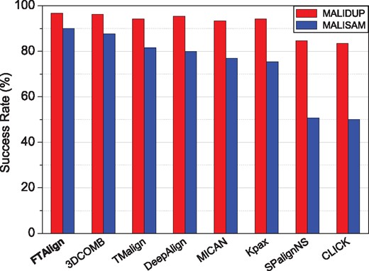
Success rates of FTAlign and seven other state-of-the-art structure alignment methods in reproducing manually curated structure alignments on two gold-standard benchmarks, MALIDUP and MALISAM
Comparing the results of MALIDUP and MALISAM also reveals that the success rates on MALIDUP are always higher than those on MALISAM for all the tested methods (Fig. 1). This is consistent with the experimental findings that MALISAM is more challenging than MALIDUP because MALIDUP consists of distant homologs while MALISAM is made up of structural analogs (Cheng et al., 2008). Another notable feature in Figure 1 is that FTAlign only lost 7.0% in success rate (i.e. 89.2% versus 96.3%) for MALISAM versus MALISDUP, compared to 8.6% for 3DCOMB (87.7% versus 96.3%), 12.7% for TMAlign (81.5% versus 94.2%), 15.4% for DeepAlign (80.0% versus 95.4%), 16.4% for MICAN (76.9% versus 93.4%), 18.8% for Kpax (75.4% versus 94.2%), 33.9% for SPalignNS (50.8% versus 84.6%) and 33.4% for CLICK (50.0% versus 83.4%). These results suggest the robustness of FTAlign in structure alignment for both distant homologs and structure analogs.
3.2 Performance on general datasets
We further evaluated the performance of FTAlign on the two manually curated benchmarks, MALIDUP and MALISAM, and four other reference-free datasets, MALIDUP-NS, MALISAM-NS, 64 difficult cases and 199 topology-different alignments by using the reference-independent criteria, , , TMscore and SO. The results with these criteria again confirmed the superior performance of FTAlign to the other seven structure alignment algorithms, which are detailed as follows.
3.2.1 Sequential datasets
Table 3a–c lists the average number of aligned residues (), RMSD of aligned residues (), TMscore of aligned residues and structure overlap (SO) for FTAlign on three sequential test sets, MALIDUP, MALISAM and 64 difficult cases, of which the SO values are also shown in Figure 2. For comparison, the table and figure also gives the corresponding results of the other seven structure alignment methods, TMalign, DeepAlign, Kpax, 3DCOMB, MICAN, SPalignNS and CLICK. It can be seen from Table 3 and Figure 2 that FTAlign achieved the highest SO on all three sequential test sets, followed by TMalign, 3DCOMB, Kpax and DeepAlign, while MICAN, SPalignNS and CLICK yielded a relatively worse performance. In addition, FTAlign obtained a higher TMscore than five of the other seven methods except TMalign and 3DCOMB. This can be understood because the two approaches TMalign and 3DCOMB have been designed to maximize the geometric similarity score (i.e. TMscore) between two protein structures during the alignment (Wang et al., 2011; Zhang and Skolnick, 2005). Given the lower success rates of TMalign and 3DCOMB than FTAlign in reproducing the manually curated alignments of MALIDDUP and MALISAM (Fig. 1), TMalign and 3DCOMB may align many more evolutionarily unrelated but geometrically similar residues than FTAlign, as also pointed out in the DeepAlign study (Wang et al., 2013). From Table 3, one can also observe that FTAlign, TMalign, 3DCOMB, Kpax, DeepAlign and MICAN obtained a significantly higher number of aligned residues than SPalignNS and CLICK, though they gave a worse average . This can be understood because the is anti-correlated with the number of aligned residues. The overall worse performances of three non-sequential alignment approaches, MICAN, SPalignNS and CLICK, than the other methods on these three sequential datasets suggest that it is challenging to develop a general approach for both sequential and non-sequential alignment, as it is unknown whether a structure alignment is sequential or not before it is manually examined. Therefore, it is encouraging that our topology-independent approach FTAlign performed the best on all the three sequential datasets.
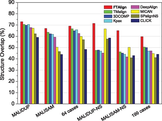
Structure overlap (SO) of FTAlign and seven other structure alignment methods on six commonly used datasets of pairwise alignments, where MALIDUP, MALISAM and 64 difficult cases are sequential sets, and MALIDUP-NS, MALISAM-NS and 199 topology-different cases are non-sequential sets
Performance comparison between FTAlign and seven other state-of-the-art methods on six test sets of pairwise structure alignments, in which MALIDUP, MALISAM and 64 difficult cases are sequential sets, and MALIDUP-NS, MALISAM-NS and 199 topology-different cases are non-sequential sets
| (a) MALIDUP | |||||||||
| Method | (Å) | TMscore | SO (%) | ||||||
| FTAlign | 87.1 | 2.68 | 0.610 | 73.0 | |||||
| Kpax | 80.1 | 2.17 | 0.609 | 70.6 | |||||
| TMalign | 86.7 | 2.69 | 0.631 | 70.4 | |||||
| 3DCOMB | 84.9 | 2.60 | 0.623 | 69.8 | |||||
| DeepAlign | 83.8 | 2.68 | 0.611 | 67.8 | |||||
| MICAN | 84.9 | 2.58 | 0.593 | 67.2 | |||||
| SPalignNS | 62.7 | 1.61 | 0.520 | 62.3 | |||||
| CLICK | 61.0 | 1.81 | 0.496 | 59.1 | |||||
| (b) MALISAM | |||||||||
| Method | (Å) | TMscore | SO (%) | ||||||
| FTAlign | 63.6 | 3.12 | 0.511 | 67.0 | |||||
| TMalign | 62.5 | 3.15 | 0.522 | 63.0 | |||||
| 3DCOMB | 60.8 | 2.97 | 0.520 | 62.3 | |||||
| Kpax | 55.9 | 2.57 | 0.493 | 61.8 | |||||
| DeepAlign | 58.9 | 3.04 | 0.500 | 59.1 | |||||
| MICAN | 61.8 | 2.99 | 0.414 | 50.5 | |||||
| SPalignNS | 35.1 | 1.82 | 0.356 | 46.4 | |||||
| CLICK | 34.8 | 1.95 | 0.346 | 44.0 | |||||
| (c) 64 difficult cases | |||||||||
| Method | (Å) | TMscore | SO (%) | ||||||
| FTAlign | 82.6 | 2.98 | 0.531 | 69.1 | |||||
| TMalign | 82.3 | 2.97 | 0.558 | 66.5 | |||||
| Kpax | 76.1 | 2.43 | 0.526 | 65.8 | |||||
| 3DCOMB | 80.9 | 2.90 | 0.540 | 64.9 | |||||
| DeepAlign | 80.8 | 3.03 | 0.533 | 62.7 | |||||
| MICAN | 79.9 | 2.90 | 0.492 | 59.8 | |||||
| SPalignNS | 57.0 | 1.78 | 0.437 | 56.9 | |||||
| CLICK | 51.0 | 1.94 | 0.380 | 48.5 | |||||
| (d) MALIDUP-NS | |||||||||
| Method | (Å) | TMscore | SO (%) | ||||||
| FTAlign | 86.0 | 2.73 | 0.597 | 71.4 | |||||
| MICAN | 83.7 | 2.55 | 0.587 | 66.6 | |||||
| CLICK | 60.4 | 1.81 | 0.493 | 58.6 | |||||
| SPalignNS | 57.8 | 1.69 | 0.477 | 57.7 | |||||
| 3DCOMB | 58.5 | 2.74 | 0.430 | 47.8 | |||||
| TMalign | 61.5 | 3.01 | 0.433 | 47.5 | |||||
| Kpax | 52.3 | 2.13 | 0.407 | 47.0 | |||||
| DeepAlign | 54.1 | 2.57 | 0.409 | 45.3 | |||||
| (e) MALISAM-NS | |||||||||
| Method | (Å) | TMscore | SO (%) | ||||||
| FTAlign | 61.8 | 3.13 | 0.498 | 65.0 | |||||
| MICAN | 61.1 | 2.96 | 0.412 | 50.3 | |||||
| TMalign | 48.3 | 3.44 | 0.393 | 45.7 | |||||
| 3DCOMB | 46.1 | 3.27 | 0.384 | 45.1 | |||||
| Kpax | 40.4 | 2.59 | 0.362 | 44.1 | |||||
| CLICK | 33.8 | 1.94 | 0.337 | 42.9 | |||||
| DeepAlign | 40.7 | 2.93 | 0.361 | 41.7 | |||||
| SPalignNS | 31.4 | 1.82 | 0.314 | 40.9 | |||||
| (f) 199 topology-different cases | |||||||||
| Method | (Å) | TMscore | SO (%) | ||||||
| FTAlign | 80.4 | 3.40 | 0.518 | 59.7 | |||||
| TMalign | 69.4 | 3.44 | 0.466 | 50.2 | |||||
| 3DCOMB | 67.3 | 3.29 | 0.462 | 50.1 | |||||
| DeepAlign | 61.6 | 3.03 | 0.433 | 47.0 | |||||
| Kpax | 57.1 | 2.62 | 0.423 | 47.0 | |||||
| MICAN | 76.8 | 3.20 | 0.418 | 44.5 | |||||
| CLICK | 46.6 | 1.99 | 0.367 | 43.7 | |||||
| SPalignNS | 42.8 | 2.00 | 0.337 | 41.1 | |||||
Note: The methods are ranked according to their SO.
3.2.2 Non-sequential datasets
Table 3d–f lists the average number of aligned residues (), RMSD of aligned residues (), TMscore of aligned residues and structure overlap (SO) for FTAlign on three non-sequential test sets, MALIDUP-NS, MALISAM-NS and 199 topology-different cases, of which the SO valuses are also shown in Figure 2. As a reference, the table and figure also gives the corresponding results of the other seven structure alignment methods, TMalign, 3DCOMB, Kpax, DeepAlign, MICAN, SPalignNS and CLICK. It can be seen from Table 3 and Figure 2 that FTAlign again obtained a better performance than the other seven structure alignment methods in terms of both SO and TMscore on the three non-sequential test sets. Several other features can also be found by comparing the results of all six test sets. First, TMalign, 3DCOMB, Kpax and DeepAlign have a significantly lower SO on the non-sequential sets than on the sequential sets. This can be understood because these four methods are designed for sequential structure alignment (Wang et al., 2013; Zhang and Skolnick, 2005). Second, MICAN maintained a comparable performance, as its algorithm is able to handle both sequential and non-sequential alignments. The SO values of SPalignNS and CLICK are relatively low on both sequential and non-sequential test sets, which may be due to their point representation of protein structures, which would lead to over-fragmentation under the pressure of minimizing the and/or maximizing the SO. On the contrary, through a global superimposition of two protein structures, FTAlign would circumvent the above limitation and thus achieved a consistently better performance than the other methods on both sequential and non-sequential test sets.
3.3 Case study
To further illustrate the advantage of a global search in structure alignment, we have investigated an example pairwise alignment, d2bs2_C1 and d2bs2_C2 from MALIDUP, on which only three methods, FTAlign, 3DCOMB and Kpax, successfully reproduced the manually curated structure alignment and gave an RMSD of <5.0 Å, while the other five methods failed to predict the manually curated alignment and led to a large RMSD of more than 20 Å (Fig. 3).
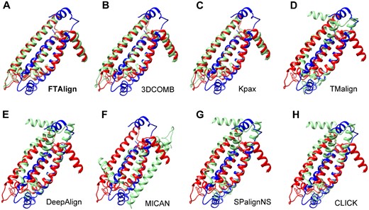
Structural comparison between the manually curated alignment (red and blue) and computationally predicted alignment (green and blue) for FTAlign (A) and seven other state-of-the-art methods (B–H) on the case of d2bs2_C1/d2bs2_C2 from MALIDUP, where the manual and predicted alignments are superimposed based on the first protein (blue) of the pair. (Color version of this figure is available at Bioinformatics online.)
The two proteins of this case are two domains of a fumarate reductase from wolinella succinogenes (PDB ID: 2BS2) (Burley et al., 2019). Further examination of all the alignment plots revealed that the failure of the other five approaches may be due to the heuristic nature of these structure alignment algorithms (Fig. 4). That is, heuristic methods always try to identify the current continuous segment(s) with the highest match score through a local greedy-like search (Ma and Wang, 2014). Therefore, these methods may get trapped in a local minimum during the search of continuous alignments. Although such a heuristic strategy can dramatically reduce the search space and speed up the alignment process, the final structure alignment will be impacted by the first identified segments. Therefore, in such situation, if the first continuous segment is a biologically wrong alignment, the final alignment will also be a biologically wrong one. This is just the case on the alignments between d2bs2_C1 and d2bs2_C2 for the five failed approaches. As shown in Figure 4, the manually curated alignment consists of two continuous segments with a medium match score, which are reproduced by FTAlign, 3DCOMB and Kpax (Fig. 4A–C). On the contrary, the five failed approaches except MICAN all contain one locally optimal continuous segment that has a higher match score than either of the two continuous segments in the manually curated alignment (Fig. 4D–H). This kind of locally optimal alignments can also be observed in the structural comparison between the manually curated and computationally predicted alignments for the failed methods (Fig. 3). As for MICAN, its failure is due to its non-sequential alignment for this sequential case, although it does not show the overfitting problem of local segments between two structures (Fig. 3F). This example suggests the necessity of developing a global structure alignment algorithm like FTAlign.
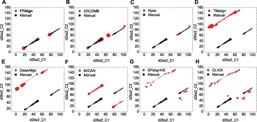
Comparison of the residue alignments between the computationally predicted (red) and manually curated (black) alignments for FTAlign (A) and seven other state-of-the-art methods (B–H) on the case of d2bs2_C1/d2bs2_C2, where the sizes of symbols are linearly scaled according to the distance between two aligned Cα atoms. Namely, a smaller symbol means a geometrically better match between two residues. (Color version of this figure is available at Bioinformatics online.)
3.4 Computational efficiency
Despite the global search process, our structure alignment method can be greatly accelerated through an FFT-based algorithm. As such, FTAlign is computationally efficient and can normally finish a pairwise alignment within seconds. Table 4 gives the total running times and average time per case of FTAlign on a single Intel(R) Xeon(R) CPU E5-2690 v4 @ 2.60 GHz core over the six test sets. For comparison, the table also lists the corresponding times of the other seven methods. It can be seen from the table that 3DCOMB is the fastest method and only consumes an average of 0.009 s for aligning a pair of structures, followed by 0.034 s for TMAlign and 0.065 s for MICAN. DeepAlign, Kpax and SPalignNS are moderately fast and can normally finish a structure alignment within a half second. FTAlign and CLICK are relatively slow and have an average running time of 2.895 and 3.906 s per case, respectively. The much higher (∼100 times) running time of FTAlign than other sequential alignment methods like TMAlign and 3DCOMB can be understood because FTAlign explores dramatically more orientational space [)] due to its exhaustive global search for an accurate topology-independent alignment. Therefore, taking its huge search space into account, FTAlign is relatively fast in some sense, though its running time is much longer than those of other sequential alignment approaches. Moreover, the FFT-based algorithm can be further speeded up through a graphic process unit (GPU). With the GPU version, a pairwise alignment can be normally completed within one second, which is fast enough for high-throughput structure alignment.
Total running times and average time per case of FTAlign and seven other methods on a single Intel(R) Xeon(R) CPU E5-2690 v4 @ 2.60 GHz core over the six test sets of pairwise structure alignments
| Method | Running time (s) | |||||||
|---|---|---|---|---|---|---|---|---|
| CLICK | FTAlign | SPalignNS | Kpax | DeepAlign | MICAN | TMalign | 3DCOMB | |
| MALIDUP | 1177.27 | 694.58 | 102.39 | 71.80 | 52.82 | 17.61 | 8.78 | 2.20 |
| MALISAM | 207.08 | 340.16 | 19.24 | 35.28 | 19.15 | 5.83 | 3.45 | 1.15 |
| 64 cases | 265.67 | 176.82 | 28.65 | 18.71 | 16.73 | 4.56 | 2.71 | 0.56 |
| MALIDUP-NS | 1140.49 | 693.46 | 95.98 | 72.32 | 49.83 | 17.21 | 8.36 | 2.20 |
| MALISAM-NS | 200.09 | 353.75 | 19.12 | 36.22 | 18.64 | 5.75 | 3.26 | 1.16 |
| 199 cases | 942.87 | 647.85 | 79.81 | 60.26 | 50.25 | 14.21 | 8.16 | 1.82 |
| Average/case | 3.906 | 2.895 | 0.344 | 0.297 | 0.208 | 0.065 | 0.034 | 0.009 |
To choose an appropriate method for real applications, both computational efficiency and alignment accuracy need to be considered. For sequential alignment, programs like TMAlign and 3DCOMB would be the ideal choice, owing to their high speed. However, for topology-independent alignment, FTAlign would be an optimal one because of its significant accuracy advantage and also acceptable running time.
3.5 Impact of alignment parameters
During our FFT-based global search for optimal alignment between two protein structures, there are two basic parameters, grid spacing for 3D translational search and angle step for 3D rotational search. To investigate the impact of these two parameters on our alignment, we have conducted an extensive evaluation of FTAlign on six test sets under the combination of four grid spacings (1.0, 1.2, 1.5 and 2.0 Å) and four angle steps (10∘, 15∘, 18∘ and 20∘). Table 5 lists the SO of FTAlign with different sets of parameters on the six test sets. It can be seen from the table that the changes of SO are very small and within 1.0% for different sets of grid spacing and angle step, suggesting the robustness of FTAlign in FFT-based global search for geometric match. This may be understood because proteins are represented by their Cα atoms in FTAlign. As the average distance between two Cα atoms is around 3.8 Å, FTAlign is expected to perform well as long as the grid spacing is significantly smaller than 3.8 Å, although we have taken the grid spacing of 2.0 Å and angle step of 18∘ as the default parameters of FTAlign for the sake of both accuracy and speed in the present study.
Structure overlaps (SO) of FTAlign with different grid spacings and angle steps on six test sets
| Grid spacing | Angle step | Structure overlap (%) | |||||
|---|---|---|---|---|---|---|---|
| MALIDUP | MALISAM | 64 cases | MALIDUP-NS | MALISAM-NS | 199 cases | ||
| 1.0 Å | 10∘ | 73.1 | 67.3 | 68.9 | 71.4 | 65.1 | 59.7 |
| 15∘ | 72.9 | 67.4 | 68.9 | 71.4 | 64.7 | 59.4 | |
| 18∘ | 72.8 | 67.2 | 68.7 | 71.5 | 64.7 | 59.8 | |
| 20∘ | 73.0 | 67.0 | 68.7 | 71.6 | 64.4 | 59.9 | |
| 1.2 Å | 10∘ | 73.2 | 67.3 | 69.1 | 71.4 | 64.7 | 59.6 |
| 15∘ | 73.0 | 67.0 | 69.0 | 71.2 | 64.8 | 59.7 | |
| 18∘ | 72.9 | 66.9 | 68.9 | 71.4 | 64.5 | 59.5 | |
| 20∘ | 72.8 | 67.1 | 68.4 | 71.4 | 64.8 | 59.5 | |
| 1.5 Å | 10∘ | 72.9 | 67.2 | 68.9 | 71.2 | 65.1 | 59.6 |
| 15∘ | 72.8 | 67.3 | 69.3 | 71.4 | 64.9 | 59.5 | |
| 18∘ | 73.0 | 67.1 | 68.8 | 71.3 | 64.7 | 59.8 | |
| 20∘ | 72.9 | 66.8 | 68.9 | 71.6 | 64.7 | 59.6 | |
| 2.0 Å | 10∘ | 73.1 | 67.2 | 69.0 | 71.3 | 64.8 | 59.5 |
| 15∘ | 73.1 | 66.9 | 68.9 | 71.5 | 64.7 | 59.8 | |
| 18∘ | 73.0 | 67.0 | 69.1 | 71.4 | 65.0 | 59.7 | |
| 20∘ | 72.8 | 66.8 | 68.7 | 71.3 | 64.6 | 59.8 | |
4 Conclusions
We have developed an accurate topology-independent and global structure alignment method based on an FFT-based search algorithm, which is referred to as FTAlign. FTAlign was extensively evaluated on six commonly used test sets including two manually curated gold-standard benchmarks, MALIDUP and MALISAM and four reference-free test sets, MALIDUP-NS, MALISAM-NS, 64 difficult cases from HOMSTRAD and 199 topology-different pairwise alignments, in which MALIDUP, MALISAM and 64 difficult cases are sequential sets and MALIDUP-NS, MALISAM-NS and 199 topology-different cases are non-sequential sets. It was shown that FTAlign not only obtained a better success rate in reproducing manually curated structure alignments on MALIDUP and MALISAM, but also achieved a higher biologically meaningful structure overlap (SO) and an overall higher TMscore on the six test sets than seven other state-of-the-art structure alignment methods, TMAlign, 3DCOMB, Kpax, DeepAlign, MICAN, SPalignNS and CLICK. A case study further confirmed the advantage of a global search like FTAlign in structure alignment. Despite its global search feature, FTAlign is also computational efficient and its GPU version can normally finish a structure alignment within one second. FTAlign provides a general method for both sequential and non-sequential alignments between two protein structures.
Funding
This work was supported by the National Natural Science Foundation of China (grant No. 31670724), the National Key R&D Program of China (grant Nos. 2016YFC1305800 and 2016YFC1305805), the National 1000 Young Thousand Talents of China and the startup grant of Huazhong University of Science and Technology.
Conflict of Interest: none declared.
References

