Non-parametric individual treatment effect estimation for survival data with random forests

Abstract

Motivation

Personalized medicine often relies on accurate estimation of a treatment effect for specific subjects. This estimation can be based on the subject’s baseline covariates but additional complications arise for a time-to-event response subject to censoring. In this paper, the treatment effect is measured as the difference between the mean survival time of a treated subject and the mean survival time of a control subject. We propose a new random forest method for estimating the individual treatment effect with survival data. The random forest is formed by individual trees built with a splitting rule specifically designed to partition the data according to the individual treatment effect. For a new subject, the forest provides a set of similar subjects from the training dataset that can be used to compute an estimation of the individual treatment effect with any adequate method.

Results

The merits of the proposed method are investigated with a simulation study where it is compared to numerous competitors, including recent state-of-the-art methods. The results indicate that the proposed method has a very good and stable performance to estimate the individual treatment effects. Two examples of application with a colon cancer data and breast cancer data show that the proposed method can detect a treatment effect in a sub-population even when the overall effect is small or nonexistent.

Availability and implementation

The authors are working on an R package implementing the proposed method and it will be available soon. In the meantime, the code can be obtained from the first author at .

Supplementary information

Supplementary data are available at Bioinformatics online.

1 Introduction

The estimation of individual treatment effect, which is of foremost importance in personalized medicine because the treatment effect can be heterogeneous in a population, is a very active area of research (Fernald et al., 2011; Wang and Dai, 2016; Zhang et al., 2017). Let Y be the outcome of interest for a subject in the population, W be the group variable indicating whether the subject is in the treatment (W = 1) or control (W = 0) group, and $\mathrm{X}$ be a vector of covariates for the same subject. The individual treatment effect (ITE) is defined by

$$\tau (\mathrm{x})=E[Y|W=1,X=x]-E[Y|W=0,X=x].$$

(1)

In (1), the outcome Y could be continuous or binary (0-1), and in the latter case, $E[Y]=P[Y=1]$⁠. The ITE measures the average treatment effect for a particular covariates pattern. The study of ITE go back a long way (Rubin, 1974) and is a causal problem; see Imbens and Rubin (2015) for a general introduction. In the business literature, the terms ‘uplift’ or ‘incremental’ modeling are used for the same problem (Hansotia and Rukstales, 2002; Lo, 2002). A recent review by Gérardy and Gutierrez (2016) classify the methods to estimate ITE into three mains approaches: The two-model approach, the class transformation approach and the direct approach. Basically, the two-model approach estimates separate models for the treatment and control groups. The class transformation approach uses a transformed outcome defined with the propensity score. The last approach uses recursive partitioning, that is tree-based methods, to model the ITE directly.

Trees are particularly useful and effective for finding subgroups of subjects with similar treatment effects since they build covariates-based partitions of the population. Moreover, they do not require to specify a priori the link between the covariates and the response. In fact, tree-based methods are able to automatically find this link, including the interactions between the covariates. Several tree-based methods for estimating ITE have been proposed, e.g. Hansotia and Rukstales (2002), Radcliffe and Surry (2011), Rzepakowski and Jaroszewicz (2012), Athey and Imbens (2015) and Thomas et al. (2018). Ensembles of trees (random forest) are among the most powerful and popular statistical learning methods (Breiman, 2001). They have also been proposed for this problem (Athey et al., 2019; Guelman et al., 2015; Sołtys et al., 2015).

However, most methods, including the ones above are aimed at uncensored outcomes. If the goal is to study the time before an event of interest (e.g. death, cancer relapse), then (right-) censored observations are likely to occur since all subjects will not have experienced the event by the time the study ends. Tree-based methods for estimating ITE with censored data have only recently been proposed. Jaroszewicz and Rzepakowski (2014) propose a general method that transforms survival data into classification data by considering a new binary outcome defined as whether or not the observed time is greater or equal than some selected threshold. Any classification method, including trees and forests, can be used with this outcome. Loh et al. (2015) show how to use the GUIDE methodology (Loh, 2002) to identify subgroups with differential treatment effects, including how to adapt it to censored data. Seibold et al. (2016) use model based recursive partitioning (Zeileis et al., 2008) to achieve the same goal. Zhang et al. (2017) develop a novel tree building algorithm called Survival Causal Tree to estimate the ITE with censored data. The main idea is to build the tree with an adjusted outcome using the propensity score and the inverse probability of censoring (Anstrom and Tsiatis, 2001). Henderson et al. (2018) extend the Bayesian Additive Regression Trees (BART) method (Chipman et al., 2010) using an accelerated failure time model to estimate the ITE with censored data.

Random forests were introduced as a way to average the predictions from many trees. However, forests are now seen as a way to generate data-driven weights that can be used to compute any desired summary for a new observation (Hothorn et al., 2004; Lin and Jeon, 2006; Moradian et al., 2017, 2019; Roy and Larocque, 2019). Basically, these weights provide a set of observations from the training dataset that are similar to the one we want to predict.

Our goal is to propose and investigate a novel and flexible way to build trees leading to a random forest to estimate the ITE with censored data. The trees are built with a new splitting rule specifically designed to partition the data according to the ITE. For a new observation, the proposed forest provides a set of similar observations from the training dataset that can be used to compute an estimation of the ITE with any appropriate method. This paper is organized as follows. The settings, assumptions and proposed method are described in Section 2. In Section 3, a simulation study compares the proposed method to generic and recent state-of-the-art methods. Real data examples are provided in Section 4, followed by concluding remarks in Section 5.

2 Proposed method

In this section, we describe in details the setting, assumptions and proposed method.

2.1 Notation and available data

We are interested in the true survival time Y. However, the observed survival time is $T=\min (Y,V)$ where V is the censoring time. We also observe the censoring indicator $\delta =I(Y\ge V)$⁠. A typical observation is thus $(T,\delta ,W,\mathrm{X})$⁠, where, as seen in the Introduction, W is the group variable indicating whether the observation is in the treatment (W = 1) or control (W = 0) group, and $\mathrm{X}$ is a vector of covariates. We assume that Y and V are independent, given the covariates $\mathrm{X}$ and the treatment indicator W. Our goal is to estimate the ITE defined by (1). The data consist in N independent observations, N^T are in the treatment group and N^C are in the control group (⁠$N=N^T+N^C$⁠).

The treatment assignment can be from a controlled experiment, or may arise from observational data. In the latter case, we assume the unconfoundedness assumption, which states that the treatment assignment is independent of the two potential outcomes (one for the treatment group and one for the control group), conditional on the covariates; see chapter 3 of Imbens and Rubin (2015).

Another representation of the ITE function will be useful for the splitting criterion described in the next section. Denote by $S^T(·|x)$ the conditional survival function of the survival time for a subject in the treatment group with covariates $x$⁠, that is, $S^T(y|x)=P(Y>y|W=1,X=x)$⁠. Similarly, denote by $S^C(·|x)$ the conditional survival function of the survival time for a subject in the control group with covariates $x$⁠, that is, $S^C(y|x)=P(Y>y|W=0,X=x)$⁠. Since the expected value of a positive random variable is equal to the integral of its survival function, we have

$$\tau (x)={\int }_0^{\infty }[S^T(y|x)-S^C(y|x)]\mathit{dy}.$$

2.2 Survival ITE tree splitting criterion

We use a random forest to estimate the ITE. This random forest is formed by survival ITE trees that are built with a special splitting criterion. We assume the reader is familiar with the basic CART algorithm (Breiman et al., 1984), as only a brief description is given here. Assume we want to split a parent node into two children nodes, call them the left and right nodes. The parent node has N_P observation, $N_P^T$ are in the treatment group and $N_P^C$ are in the control group (⁠$N_P=N_P^T+N_P^C$⁠). To split a node, all allowable splits (see Supplementary Material for details) are evaluated, using the observations in the parent node only, and the best one is selected according to a specific criterion. For a continuous or ordinal covariate X, we create splitting variables $\eta =I(X\le \upsilon )$ where $\upsilon$ is the midpoint between two consecutive distinct values of X. For a categorical covariate, we create splitting variables $\eta =I(X\in \{{\upsilon }_1,{\upsilon }_2,\dots ,{\upsilon }_q\})$ where $\{{\upsilon }_1,{\upsilon }_2,\dots ,{\upsilon }_q\}$ is a subset of the possible values of X. Once the best split is found, the parent node observations with η = 0 go to the left node, and the ones with η = 1 go to the right node.

Define ${\widehat{\tau }}_L$ and ${\widehat{\tau }}_R$ to be the estimated ITE in the left and right nodes, respectively. The specific way to get these estimates is described below. The main idea motivating the proposed splitting criterion is that we want to increase the heterogeneity of the ITE estimates as fast as possible. That is, we want $|{\widehat{\tau }}_L-{\widehat{\tau }}_R|$ to be large. In the case of a binary response without censoring, this criterion was proposed in Hansotia and Rukstales (2002). However, as recognized by Radcliffe and Surry (2011), this criterion does not take into account the size of the children nodes, which has the effect of neglecting the precision of the ITE estimations. Following Moradian et al. (2017), we instead propose

$$\Delta \tau =\sqrt{N_L{N}_R}|{\widehat{\tau }}_L-{\widehat{\tau }}_R|,$$

(2)

as the splitting criterion, where N_L and N_R are the left and right node sizes, respectively. The best split is the one maximizing (2) among all allowable splits. The factor $\sqrt{N_L{N}_R}$ penalizes unbalanced splits, that is splits where the estimated ITE is based on a small number of observations.

The estimates ${\widehat{\tau }}_L$ and ${\widehat{\tau }}_R$ can be obtained in many ways. However, we require a way that is relatively quick to compute because it will need to be evaluated many times, that is for each allowable split in each node of each tree. For a candidate split, define ${\widehat{S}}_L^T$ and ${\widehat{S}}_L^C$ to be the Kaplan–Meier estimate of the observations in the treatment group in the left node, and the Kaplan–Meier estimate of the observations in the control group in the left node, respectively. Define ${\widehat{S}}_R^T$ and ${\widehat{S}}_R^C$ as the same quantities in the right node. The estimated ITE in the left node is given by

$${\widehat{\tau }}_L={\int }_0^{\infty }[{\widehat{S}}_L^T(y)-{\widehat{S}}_L^C(y)]\mathit{dy}.$$

(3)

Similarly, the estimated ITE in the right node is given by ${\widehat{\tau }}_R={\int }_0^{\infty }[{\widehat{S}}_R^T(y)-{\widehat{S}}_R^C(y)]\mathit{dy}$⁠. Consequently, the proposed splitting rule (2) has an explicit formula, and the split controls described in the next section will ensure that it is well defined. There is one last technical point however. The Kaplan–Meier estimate can be undefined past a certain value, for instance when the largest observed time is censored. In that case, we add a tail to the Kaplan–Meier curve to be able to compute the integral up to infinity. The details are provided in Supplementary Material.

The procedure for building the tree is similar to the CART algorithm. We start at the root node containing all observations. We evaluate all allowable splits. If no allowable split is available, then the node becomes terminal. If at least one split is allowable, then we split the node according to the best one, that is the one maximizing (2). We repeat the process with the left node and then the right node. The tree building process ends when all nodes are terminal.

2.3 Random forest and ITE estimates

The last section described the splitting rule that we use to build a single tree. However, the final ITE estimate is based on a random forest (RF). The original RF algorithm (Breiman, 2001) can be described by a simple algorithm.

For $b=1,\dots ,B$

1. Draw a boostrap sample of the original data.

2. Grow a tree (usually unpruned) using the bootstrap data with the following modification. At each node, rather than choosing the best split among all predictors, randomly sample p₀ (⁠$0<p_0\le p$⁠) of the p predictors and choose the best split among those variables.

3. Compute the predictions by averaging in some way the predictions of the individual trees.

For example, for a regression forest with a continuous response Y, the final RF prediction for a new observation with covariate vector $x_{\mathit{new}}$ is the average of the individual tree predictions

$${\widehat{y}}_{\mathit{RF},\mathit{new}}=\frac{1}{B}\sum _{b=1}^B{\widehat{y}}_{b,\mathit{new}},$$

where ${\widehat{y}}_{b,\mathit{new}}$ is the prediction from the $b^{\text{th}}$ tree. However, the modern way to view a forest is as a way to obtain observation weights. Indeed, we can also write the RF prediction above as a weighted average of the training observations

$${\widehat{y}}_{\mathit{RF},\mathit{new}}=\sum _{i=1}^n{\widehat{w}}_i(x_{\mathit{new}})y_i,$$

where the y_i are the original observations and the w_i are weights. This is easy to see since ${\widehat{y}}_{b,\mathit{new}}$ is the average of the observations in the terminal node where $x_{\mathit{new}}$ ends up. These weights were used in a survival data setting by Hothorn et al. (2004) and were named ‘nearest neighbor forest weights’ by Lin and Jeon (2006).

In this paper, we use a slightly different version of these weights introduced in Moradian et al. (2017), and then used in Moradian et al. (2019) and Roy and Larocque (2019). The main idea is to use the pooled set of training observations that are in the same terminal nodes as $x_{\mathit{new}}$ in the forest. This set is called Bag of Observations for Prediction or simply BOP in Roy and Larocque (2019). More formally, let $S_b(x_{\mathit{new}})$ be the training responses that are in the same terminal node as $x_{\mathit{new}}$ for the $b^{\text{th}}$ tree. The BOP for $x_{\mathit{new}}$ is

$$\text{BOP}(x_{\mathit{new}})=\bigcup _{b=1}^B{S}_b(x_{\mathit{new}}).$$

The idea is to use $\text{BOP}(x_{\mathit{new}})$ to compute any desired summary for this new observation. In our case, $\text{BOP}(x_{\mathit{new}})$ is used to estimate the ITE. If we use appropriate split control parameters, then $\text{BOP}(x_{\mathit{new}})$ contains observations from both the treatment and control groups. Hence, we can estimate the expected value of each group separately, and take the difference to estimate the ITE. More precisely, let ${\widehat{S}}^T(y|x_{\mathit{new}})$ be the Kaplan–Meier estimate of the survival function computed with the treatment observations in $\text{BOP}(x_{\mathit{new}})$⁠. Similarly, let ${\widehat{S}}^C(y|x_{\mathit{new}})$ be the Kaplan–Meier estimate of the survival function computed with the control observations in $\text{BOP}(x_{\mathit{new}})$⁠. The forest ITE estimates is obtained from

$${\widehat{\tau }}_{\mathit{RF}}(x_{\mathit{new}})={\int }_0^{\infty }[{\widehat{S}}^T(y|x_{\mathit{new}})-{\widehat{S}}^C(y|x_{\mathit{new}})]\mathit{dy}.$$

(4)

2.4 Implementation

The heavy computational part of the proposed method is to build the trees to get a forest. The new tree building algorithm is coded in C++, callable from R (R Core Team, 2017). We are working on an R package implementing the proposed method. It should be available soon.

3 Simulation study

Evaluating an ITE model with real data is not a simple task. For the basic supervised learning problem with a single response, we can calculate the difference between the real value of the response and the model prediction over a holdout dataset. In the case of ITE modeling, the true ITE is unknown because each subject is only in one of the treatment or the control group. Therefore, we use a simulation study to validate our approach in this section. Real data applications are provided in the following section. In a simulation context with a fully know Data Generating Process (DGP), we know the true underlying ITE and we can measure the performance of a model based on them. We compare our method to three generic methods and to four methods proposed in the literature.

3.1 Competing methods

The first model is an application of the Lo (2002) methodology. The second and third models are applications of the two models approach of Hansotia and Rukstales (2002). The fourth and fifth are state-of-the art methods proposed in Henderson et al. (2018) and Zhang et al. (2017). The sixth and seventh methods are two versions of the Jaroszewicz and Rzepakowski (2014) binary transformation method.

3.1.1 AFT interaction model

To get ITE estimates with a binary response, Lo (2002) used a logistic regression model in which he includes all the covariates, the binary treatment indicator and all interactions between this indicator and the covariates. A simple adaptation of this idea to our setting is to use an accelerated failure time (AFT model), instead of a logistic regression. Using the original data, we fit the model

$$T=\text{exp}({\beta }_0+X\prime {\beta }_1+W{\beta }_2+X\prime W{\beta }_3)ϵ,$$

(5)

for many choices of error distribution, and we select the distribution with the best value of the AIC criterion. This distribution becomes the working distribution used to compute the ITE estimates for new observations. In this article, the function survreg in the survival package (Therneau, 2015) is used, and we determine the distribution empirically. For each dataset, we fit models with the following distributions: Weibull, exponential, Gaussian, logistic, lognormal, loglogistic. The one retained is the one that minimizes the AIC. To get the ITE estimates once the model is fitted, we take the dataset to score, and add a new variable W. We set it to 1 to get the expected survival time estimates for the treatment group from our fitted model through the R predict function. We set W to 0 to get the expected survival time estimates for the control group. The estimated ITE is calculated by subtracting the control group estimation from the treatment group estimation for each observation.

3.1.2 Two-AFT (2AFT) model

Instead of using a single model with interactions between the treatment indicator and the covariates, another related method consists in fitting two separate AFT models, one for the treated observations and one for the control ones. The expected survival time can be obtained with the R predict function separately from the two fitted models. The estimated ITE is calculated by subtracting the control group estimation from the treatment group estimation for each observation. We use the same distribution as the one used for the AFT interaction model.

3.1.3 2 random forests (2RF) model

This method builds two separate survival forests, one for the treatment group and one for the control group. The function rfsrc in the R package randomForestSRC (Ishwaran and Kogalur, 2017) is used with the default logrank splitting rule, and 100 trees are built for each forest. This package does not provide directly estimated expected survival times for new data. But we can use the same approach as for the proposed method. To obtain the ITE estimates for a new observation, we first get its two BOPs, one from the treatment forest and one for the control forest. Using these BOPs, we can compute the Kaplan–Meier estimates of the control and treatment observations and get the ITE estimate using (4).

3.1.4 BAFT

This method is described in Henderson et al. (2018) and is an extension of the BART method to censored data. The code is available in the R package AFTrees (https://github.com/nchenderson/AFTrees).

3.1.5 Survival Causal Forest (SCF)

This method is described in Zhang et al. (2017). The code is available in the R package SurvivalCausalTree (https://github.com/WeijiaZhang24/SurvivalCausalTree). The method described in the article uses only one tree. To be more coherent with our work, we create 100 unpruned trees with bootstrap samples. The final prediction is the average of the 100 trees predictions.

3.1.6 TM model

This is a first version of the method proposed in Jaroszewicz and Rzepakowski (2014). It is based on the binary transformed outcome $Z=I(T\ge \theta )$⁠, where θ is a threshold selected by the analyst. Any classification method can be used to model Z. To be coherent with the rest of the paper, we use a random forest. Unless a secondary censoring model is used, this method does not provide an estimated ITE. However, if we assume that the censoring distribution does not depend on the covariates, and it is the case in the scenarios of this simulation study, then it can provide a ranking of the observations in terms of the ITE. In this first version, we set θ equal to the median survival time for the DGP.

3.1.7 T3Q model

This method is the same as the one just described before (TM model) but it uses the third quartile of the survival time instead of the median. This is the second version of the Jaroszewicz and Rzepakowski (2014) method. Again, it only provides a ranking of the observations and not an estimate of the ITE.

3.2 Simulation design

The main advantage of using simulations with known DGPs is that we know exactly the true ITE value, and we can use it to assess the performance of the methods. Five different DGPs (described in Supplementary Material) are used to generate true survival times Y as a function of a vector of covariates $X$⁠. We consider four different censoring proportions: 0, 20, 40 and 60%. Censoring is introduced by generating an exponentially distributed random variable V with mean $1/\alpha$⁠. The parameter α controls the proportion of censoring. For each DGP, α was found empirically to give the desired censoring proportion. The observed time T is created as $\min (Y,V)$⁠, and the censoring indicator is $\delta =I(Y\ge V)$⁠. The observed data used to build the models is a sample of $(T,\delta ,W,X)$⁠. We use training sample sizes of n_train = 500 and n_train = 1000, and we also investigate if the proportion of treatment observations has an impact. We first consider the balanced case with a 50% treatment and 50% control proportions. However, in many real applications, there are less treatment observations than control ones. This is why we also consider the case of 25% treatment and 75% control. In all, these combinations produce 40 scenarios (5 DGPs × 4 censoring proportions × 2 proportions of treatment observations) with a training sample size of 500 and another 40 scenarios with a training sample size of 1000, for a total of 80 scenarios. Each scenario is repeated 100 times for a total of 8000 total runs. For each run, an independent test set with n_test = 1000 new observations are generated according to the corresponding DGP, and is used to evaluate the performance using two criteria. The first one is the mean squared error (MSE) between the ITE estimates and the true ITE. That is, let ${\widehat{\tau }}_i$ and τ_i denote the estimated (for a given method) and true ITE for the ith observation in the test set for a given run. The MSE for this method for this run is:

$$\mathit{MSE}=\frac{1}{n_{\mathit{test}}}\sum _{i=1}^{n_{\mathit{test}}}{({\widehat{\tau }}_i-{\tau }_i)}^2.$$

Smaller values of the MSE indicate better methods. The MSE is essentially a calibration criterion, as it measures the similarity between the actual and estimated values. The second criterion is the well-known C-index (or Concordance index) (Harrell et al., 1982). The C-index value for a method is the proportion of pairs of observations, among all pairs, that are ordered correctly in terms of the ITE. Larger values of the C-index indicate better methods. It is a discriminant criterion as it measures if the estimated values are in the right order; see Riccardo et al. (2014) for a discussion about calibration and discriminant measures. Since the C-index only requires a ranking of the observations, it can be used to evaluate the performance of the TM and T3Q methods, for which the MSE is not available. Complex DGPs are used to show the ability of forest based methods to uncover the link between the covariates and the response. A detailed description of the five DGPs is given in Supplementary Material.

3.3 Simulation results

We provide a general summary of the results here. A detailed discussion about the results for each individual DGP is given in Supplementary Material. There are 100 simulation runs per scenario. In a given run, we can compute the % increase in MSE with respect to the best performer for this run, for the six methods that provide estimates of the ITE, that is all methods except TM and T3Q. These two methods provide only a ranking and their performance will be evaluated with the C-index. Note that the best performer varies from one run to another. This procedure allows us to compare the results across all scenarios all at once. More precisely, for a given run, let ${\text{MSE}}_i$ (⁠$i=1,2,\dots ,6)$ be the MSE for the ith method and ${\text{MSE}}_{\text{min}}=\min \{{\text{MSE}}_1,\dots ,{\text{MSE}}_6\}$ be the best (smallest) MSE for this run. The % increase in MSE of method i with respect to the best is given by (⁠${\text{MSE}}_i$/${\text{MSE}}_{\text{min}}$ − 1)×100. For a given run, if there are no tied MSE, one and only one method will get a % increase of 0 (the best one) and the others will get positive values. Figure 1 presents the box-plots of this metric for all methods over all 4000 runs with a training size of 1000. The methods are presented in the following order: Proposed method (ITE SRF), AFT interaction model (Interaction), Indirect model with 2RF, Bayesian Accelerated Failure Time (BAFT), Survival Causal Forest (SCF) and 2AFT model. We see that the proposed method and the BAFT method globally outperform the other ones. The proposed method has the smallest median and mean percent increase in MSE.

Fig. 1.

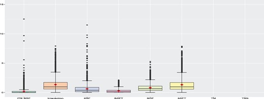
Global simulation results when the training sample size is 1000. The box-plots represent the distribution of the % increase in MSE with respect to the best performer for each run for all 4000 runs. Smaller values are better. The TM and T3Q methods only provide rankings and the MSE cannot be computed

Using the C-index, we can also compare each method to the best performer for a given run. The C-index is available for all eight methods. Since larger values of the C-index are better, we compute the % decrease in C-index with respect to the best performer for each run, for the eight methods. More precisely, for a given run, let ${\text{CI}}_i$ (⁠$i=1,2,\dots ,8)$ be the C-index for the ith method and ${\text{CI}}_{\text{max}}=\max \{{\text{CI}}_1,\dots ,{\text{CI}}_8\}$ be the best (largest) C-Index for this run. The % decrease in C-Index of method i with respect to the best is given by (⁠$1-{\text{CI}}_i$/${\text{CI}}_{\text{max}}$⁠)×100. Figure 2 presents the box-plots of this metric for all methods over all 4000 runs with a training size of 1000. As with the MSE criterion, we see that the proposed method and the BAFT method globally outperform the other ones. The T3Q method globally performs better than TM. Hence, in this study, it is better to use the third quartile as the threshold rather than the median. The T3Q method performs slightly better than the SCF method. The results when using a training sample size of n_train = 500 are presented in Supplementary Material and are very similar. A detailed discussion for individual DGPs is provided in Supplementary Material.

Fig. 2.

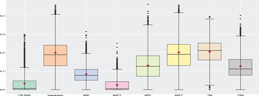
Global simulation results when the training sample size is 1000. The box-plots represent the distribution of the % decrease in C-Index with respect to the best performer for each run for all 4000 runs. Smaller values are better

4 Real data example

In this section, we illustrate the use of the proposed method with two well-known datasets. In the first one there is no significant treatment effect for the whole sample. In the second one, the treatment variable is significant for the whole sample.

4.1 The colon cancer dataset

The dataset contains the results of trials of adjuvant chemotherapy for colon cancer and is available in the survival package in R. It contains two different chemotherapy treatments. The first one is levamisole and the second one is levamisole combined with 5-FU (fluorouracil). There are two event types: disease recurrence and death. The dataset contains 16 variables and 1858 observations, two per subject, one for recurrence and one for death. In this study, we only use levamisole as treatment and death as the event of interest. When selecting these observations, we have 625 observations. After removing observation with missing data values, we end up with 599 observations that we use for this example. All the following results and discussions are about this subset of the data. The censoring rate is 47.7% and we have 49.1% of treated observations. The response (time) is the time to death or until censoring. The censoring is indicated by the status variable (1 = event, 0 = censored). The binary treatment variable is rx (’Lev’ for treatment and ’Obs’ for control). There are 10 covariates: sex (0 = female, 1 = male), age (in years), obstruct (obstruction of colon by tumor), perfor (perforation of colon), adhere (adherence to nearby organs), nodes (number of lymph nodes with detectable cancer), differ (differentiation of tumor on an ordinal scale; 1 = well, 2 = moderate, 3 = poor), extent (extent of local spread on an ordinal scale; 1 = submucosa, 2 = muscle, 3 = serosa, 4 = contiguous structures), surg (time from surgery to registration; 0 = short, 1 = long) and node4 (are there more than 4 positive lymph nodes; 0 = non, 1 = yes). More details are available in Laurie et al. (1989), Lin (1994), Moertel et al. (1990) and Moertel et al. (1995).

4.2 German Breast Cancer Study Group 2 dataset

German Breast Cancer Study Group is a study of effectiveness of two different hormonal breast cancer treatments. It is available in the TH.data (Hothorn, 2017) package in R. This study was conducted on 686 women from 21 to 80 years old on which they reported the recurrence-free time. 56.4% of the observations are censored and 35.8% received the treatment. There are no missing data. The response (time) is the recurrence free time or time until censoring in days. There are seven covariates: age (in years), menostat (menopausal status, pre/post), tsize (tumor size in mm), tgrade (tumor grade on a scale from 1 to 3), pnodes (number of positive nodes), progrec (progesterone receptor in fmol) and estrec (estrogen receptor, in fmol). Censoring is indicated with the covariate cens. The binary treatment variable is horTh (‘yes’ for hormonal treatment and ‘no’ for control). More details are available in Schumacher et al. (1994) and Sauerbrei and Royston (1999).

4.3 Data analysis

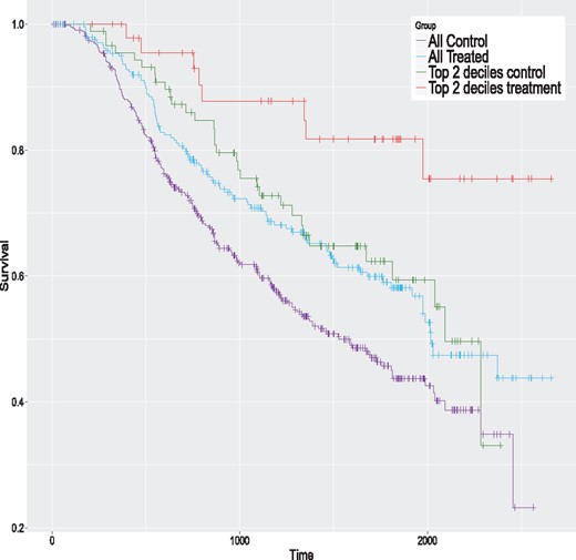
We begin with the colon cancer data. We first fit an AFT model with the lognormal distribution to the complete dataset (599 observations). This distribution is selected because it is the one with the smallest AIC value. Table 1 presents the estimated model. The treatment variable (rx) is not significant. The Kaplan–Meier curves of the control and treatment groups for the complete sample are given in Figure 3 (the two lowest curves). Clearly, the two groups have a similar survival pattern, and no global treatment effect seems apparent.

Fig. 3.

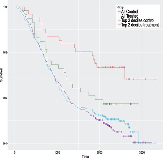
Kaplan–Meier curves for the colon data for the whole sample and the top 2 ITE deciles for the proposed method

Table 1.

AFT model (lognormal dist.) with the colon cancer dataset (N = 599)

Variable	Beta	SE	P-values
Intercept	10.7543	0.5320	0.0001
Sex	−0.1382	0.1098	0.2080
Age	−0.0140	0.0046	0.0023
Obstruct	−0.3859	0.1331	0.0038
Perfor	−0.0744	0.2972	0.8020
Adhere	−0.0791	0.1499	0.5980
Nodes	−0.0473	0.0210	0.0240
Differ	−0.1703	0.1062	0.1090
Extent	−0.4648	0.1277	0.0003
Surg	−0.2049	0.1197	0.0868
node4	−0.6956	0.1767	0.0001
rx (treatment)	−0.0049	0.1082	0.9640

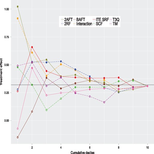
We apply the same eight methods considered in the simulation study to this dataset using the same control parameters. However, to get valid ITE estimates, we do in with a 20-fold cross-validation scheme; see Simon et al. (2011) for a related method. Simply applying the method to the complete dataset and computing the ITE with the same data would produce over-optimistic values. More precisely, the data are randomly partitioned into 20 groups of nearly equal size. One at a time, we remove each group and apply models to the sample consisting of the remaining groups, that is to 95% of the data. The fitted models are used to compute the estimated ITE for the left-out group (5% of the data). Hence, we build each model 20 times. In the end, each observation has a single ITE estimate per method, obtained when this observation is in the left-out group. For each method, the estimated ITE are ranked from the largest to the smallest values and grouped in deciles. For a given method, the first decile contains the top 10% of observations with the largest estimated ITE. The second decile contains the next 10% of observations and so on. The tenth decile contains the 10% of observations with the smallest ITE. For each method, we fit AFT models to samples formed by consecutive cumulated deciles. The first model is fit using the first decile only (10% of the data). The second model is fit using the first two deciles (20% of the data), and so on. The last model is fit to the whole sample (100% of the data) and is equivalent to the model presented in Table 1. The results are summarized in Figure 4. This figure provides the estimated treatment effects of all these models. A filled dot means that the treatment effect is significantly greater than 0 (one-sided test) and an empty one indicates a non-significant difference. The P-values should be interpreted with caution and mostly as a descriptive tool, since we are in a ‘inference after model selection’ situation. We see that the largest estimated effects occur for models with samples formed by either the top ITE decile or the top 2 ITE deciles. Three of them are significantly larger than 0. The ones of the proposed method for the top ITE decile and the top 2 ITE deciles, and the one of the TM method for the top 2 ITE deciles. This shows that the proposed and TM methods are able to identify the subjects that could potentially benefit the most from the treatment. The Kaplan–Meier curves of the control and treatment groups for the top 2 deciles of the proposed method are given in Figure 3 (the two highest curves). The global survival rate of this subsample is better than the one of the whole sample. But the treatment group has a better survival rate than the control group for this subsample, which is precisely what we want to detect. Hence, the people that are likely to benefit the most from the treatment are people that have initially a better survival rate. The treatment increases their survival rate even further. This example shows that we can detect a treatment effect in a sub-population even when the overall effect is small or nonexistent.

Fig. 4.

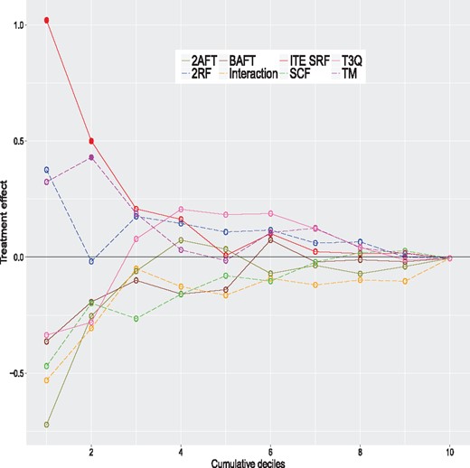
Estimated treatment effects for models fitted on cumulative deciles for the colon cancer data. A filled dot means that the treatment effect is significantly greater than 0 (one-sided test) and an empty one indicates a non-significant difference

We apply the same methodology to the German breast cancer data. We fit an AFT model with the lognormal distribution (selected with the AIC criterion) to the complete dataset (686 observations). Table 2 presents the estimated model. This time, the treatment variable (horTh) is significant (⁠$\widehat{\beta }=0.309$⁠). The Kaplan–Meier curves of the control and treatment groups for the complete sample are given in Figure 5. The estimated treatment effects for the models fitted on cumulative deciles are given in Figure 6. As for the colon data, the largest estimated effects occur for models with samples formed by either the top ITE decile or the top 2 ITE deciles. In this case, most of the effects are significantly different than 0 because there is a global treatment effect, shown with a vertical line at 0.309. The Interaction and 2AFT models detect the largest treatment effect for their top ITE deciles. As for the colon data, the proposed method has the largest treatment effect for its top 2 ITE deciles. Even though the treatment has a significant global effect, some methods are able to identify the subjects that could potentially benefit the most from the treatment. The Kaplan–Meier curves of the control and treatment groups for the top 2 deciles of the proposed method are given in Figure 5 (the two highest curves). As for the colon data, the global survival rate of this subsample is better than for the whole sample. But the treatment group has a better survival rate than the control group. More details, including Kaplan–Meier curves for all methods, are provided in Supplementary Material.

Fig. 5.

Kaplan–Meier curves for the GBSG2 data for the whole sample and the top 2 ITE deciles for the proposed method

Fig. 6.

Estimated treatment effects for models fitted on cumulative deciles for the German breast cancer data. A filled dot means that the treatment effect is significantly greater than 0 (one-sided test) and an empty one indicates a non-significant difference

Table 2.

AFT model (lognormal distr.) with the GBSG2 dataset (N = 686)

Variable	Beta	SE	P-values
Intercept	7.6127	0.3689	0.0000
Age	0.0125	0.0069	0.0698
menostat	−0.2598	0.1431	0.0696
tsize	−0.0061	0.0031	0.0516
tgrade	−0.2561	0.0818	0.0018
pnodes	−0.0504	0.008	0.0000
progrec	0.0014	0.0003	0.0001
estrec	0.0000	0.0003	0.8855
horTh (treatment)	0.3090	0.0972	0.0015

5 Concluding remarks

In this paper, we propose and study a new random forest method for estimating the ITE with censored data. This method is based on trees build with a new splitting rule specifically designed for this problem. The forest is used to obtain the BOP (Bag-of-Observations for Prediction) from which an estimated ITE can be computed using any desired method. This is the modern way to effectively use the random forest paradigm. That is, to view the forest as a data-driven way to obtain a set of observations similar to the one we want to predict. The proposed method is very flexible and amenable to various generalizations and extensions. One of them is to consider the restricted mean survival time (RMST). The RMST has received a lot of attention recently as an interesting alternative to the hazard ratio to estimate treatment effects (Horiguchi et al., 2018; Royston and Parmar, 2013). The RMST has also been used as an alternative to the (unrestricted) mean to measure the ITE (Andersen et al., 2017; Wey et al., 2016). For a given fixed value m (usually of clinical importance), the RMST of a survival response Y is defined by $E[\min (Y,m)]$⁠. The restricted individual treatment effect (RITE) can be defined as

$${\tau }^m(x)=E[\min (Y,m)|W=1,X=x]-E[\min (Y,m)|W=0,X=x].$$

The proposed splitting rule (2) can be modified to

$$\sqrt{N_L{N}_R}|{\widehat{\tau }}_L^m-{\widehat{\tau }}_R^m|,$$

where ${\widehat{\tau }}_L^m$ is the estimated RITE in the left node given by

$${\widehat{\tau }}_L^m={\int }_0^m[{\widehat{S}}_L^T(y)-{\widehat{S}}_L^C(y)]\mathit{dy},$$

and where ${\widehat{\tau }}_R^m$ is the estimated RITE in the right node defined similarly. This modified splitting rule is specifically designed for the RITE. The resulting forest would produce BOPs that can be used to estimate the final RITE. In fact, the ITE is the particular case of the RITE when $m=\infty$⁠. An in-depth investigation of this extension is left for future work. Even more generally, to detect a treatment effect in a specific time interval, say the interval $[a,b]$⁠, a specialized splitting rule can be designed in the same way, by integrating the survival curve on this interval only. In this article, we define the ITE based on the mean survival time. Other ways are possible, for example the survival probability at a given predetermined time θ, $P(Y>\theta )$⁠. The ITE can be defined as the difference $P[Y>\theta |W=1,X=x]-P[Y>\theta |W=0,X=x]$⁠. In a sense, this becomes a degenerate case of the previous generalization where we integrate the survival curve at a single point. It would also be interesting to investigate such a way to define the ITE. Finally, integrating the Kaplan–Meier faces the problem that it is sometimes undefined past a certain value. In this article, we add an exponential tail to the curve when this happens, but other methods are possible. It would be interesting to investigate how sensitive are the results with respect to the tail augmentation method chosen.

Acknowledgements

The authors want to thank the Associate Editor and two anonymous reviewers for their relevant and constructive comments and suggestions that lead to an improved version of this article.

Funding

This research was supported by the Natural Sciences and Engineering Research Council of Canada (NSERC), and by Fondation HEC Montréal.

Conflict of Interest: none declared.